The Minimax Rate of Online Isotonic Regression on Product Orders
(NeurIPS 2026), accepted
Kotłowski et al. (NeurIPS 2017) posed as a central open problem the design of efficient online isotonic regression algorithms beyond totally ordered domains. We resolve this on the product orders $[m]^d = \{1, \ldots, m\}^d$ for every fixed dimension $d \geq 2$, determining the squared-loss minimax regret over $T$ rounds up to constant factors:
$$ R_T^{*}\bigl([m]^d\bigr) \;=\; \Theta_d\!\left(\min\!\left\{T,\; \inf_{K \in \mathbb{N}_+}\!\Bigl[\, 2\, H_{[m]^d}(K) \,+\, \frac{T}{4 K^2} \,\Bigr]\right\}\right), $$where the order polynomial $\Omega(\mathcal{P}, K{+}1)$ counts the monotone maps from a poset $\mathcal{P}$ to $\{1, \ldots, K{+}1\}$ and $H_{\mathcal{P}}(K) := \log \Omega(\mathcal{P}, K{+}1)$. The formula reveals a three-phase scaling law: $\Theta_d(T)$ for $T \lesssim_d m^{d-1}$, $\Theta_d(m^{2(d-1)/3}\, T^{1/3})$ for $m^{d-1} \lesssim_d T \lesssim_d m^{d+2}$, and $\Theta_d(m^d \log(T/m^{d+2}))$ for $T \gg_d m^{d+2}$. The characterization covers every smooth, exp-concave, strongly proper, bounded loss and the entropic loss, up to loss-dependent constants, while absolute and pinball losses obey a square-root law. We construct polynomial-time algorithms matching the characterization in every regime, for every fixed $d$ and every covered loss, including a horizon-free learner requiring no advance knowledge of $T$.
1 Introduction
In online isotonic regression, a learner faces an adversary over a finite partially ordered domain: at each of $T$ rounds the learner observes a query point, predicts $\hat{y}_{t}\in[0,1]\text{,}$ and incurs the squared loss $(\hat{y}_{t}-y_{t})^{2}$ once the label $y_{t}\in[0,1]$ is revealed; its regret is the cumulative loss minus that of the best isotonic function in hindsight, nondecreasing along the partial order. On the chain, the totally ordered case, Kotłowski et al. (2016) determined the minimax regret up to logarithmic factors; beyond it, Kotłowski et al. (2017) posed the design of efficient algorithms as a central open problem, and no $\Theta$-level resolution has appeared since. This paper settles the problem on the product orders $[m]^{d}=\{1,\ldots,m\}^{d}\text{,}$ for every fixed dimension $d\geq 2\text{:}$ the minimax regret is characterized at the $\Theta$ level, the characterization is matched in polynomial time, and both statements hold across a family of losses whose boundary we locate. Queries may recur, relaxing the earlier protocols in which each point arrives once (Kotłowski et al., 2016, 2017), a choice natural for streaming (Section 2.1); Section 6 compares the protocols.
Applications.
Two scenarios motivate the multivariate setting. Two-feature probability calibration is the multivariate form of classical isotonic calibration (Zadrozny and Elkan, 2002; Niculescu-Mizil and Caruana, 2005; Berta et al., 2024): the calibrated probability of a deployed classifier is jointly nondecreasing in the model score and in an ordinal covariate. Its natural loss, the entropic (log) loss, is part of the characterization. On UCI Adult, learning on the score-by-covariate grid beats both calibration along the score alone and an unstructured per-cell mean on 20 of 20 splits (Appendix A). In combination dose-finding, the toxicity probability of a two-agent therapy is monotone in each dose, and the surface is learned along the treatment trajectory (Conaway et al., 2004; Wages et al., 2011).
Main results.
The minimax regret under squared loss is, for every fixed $d\geq 2$ and all integers $m\geq 2\text{,}$ $T\geq 1$ (Theorem 2),
| $$R_{T}^{*}\bigl([m]^{d}\bigr)\;=\;\Theta_{d}\!\left(\min\!\left\{T,\;\inf_{K\in\mathbb{N}_{+}}\!\Bigl[\,2\,H_{[m]^{d}}(K)\,+\,\frac{T}{4K^{2}}\,\Bigr]\right\}\right),\quad H_{\mathcal{P}}(K)\;:=\;\log\Omega(\mathcal{P},K{+}1),$$ |
where, for a finite poset $\mathcal{P}\text{,}$ $\Omega(\mathcal{P},N)$ counts the order-preserving maps into $\{1,\ldots,N\}\text{,}$ the order polynomial of Stanley (1970). The formula balances the two costs of learning on the value grid $\{0,1/K,\ldots,1\}\text{:}$ $H_{[m]^{d}}(K)$ is, up to a factor of two in the resolution, the sup-norm metric entropy of the comparator class, and $T/(4K^{2})$ is the cost of rounding the hindsight optimum onto the grid once its first-order term is canceled (Section 2). It unfolds into a three-phase law (Corollary 3): $\Theta_{d}(T)$ for $T\lesssim_{d}m^{d-1}$ (Phase 0); $\Theta_{d}(m^{2(d-1)/3}\,T^{1/3})$ for $m^{d-1}\lesssim_{d}T\lesssim_{d}m^{d+2}$ (Phase 1); and $\Theta_{d}(m^{d}[1+\log(T/m^{d+2})])$ beyond (Phase 2), where the grid has decoupled into $m^{d}$ scalar estimation problems. The upper bound in the display holds on every finite poset and, with loss-dependent constants, for every smooth exp-concave loss (Theorem 1); the grids are where we match it. Rectangles $[a]\times[b]$ add a fourth sector that the substitution $m\mapsto\sqrt{ab}$ misses, and the characterization persists at every fixed aspect ratio (Proposition 66). The intermediate phase carries no logarithmic factor; on the chain it does (Theorem 46), and Section 2.2 traces the difference to the entropy at coarse scales.
The law is stable in the loss: every smooth, exp-concave, strongly proper, bounded loss obeys the same characterization, and so does the entropic loss of calibration, the loss entering only through the constants (Theorem 2). Absolute and pinball losses change the rate: they obey a square-root law in which resolution plays no part, $\Theta_{d}(\min\{T,\sqrt{m^{d-1}T}\})$ for the absolute loss (Theorem 56). On the algorithmic side, two complementary planar engines (Column-Independent Chain EW and Surrogate Threshold-Indexed EW), a rate-doubling wrapper, and a slicing step combine into a horizon-free polynomial-time learner, rate-optimal for every loss of the Theorem 2 family and every fixed dimension (Theorem 7).
Technical contributions.
The characterization rests on a small set of mechanisms. For the upper bound, the isotonic fit is stationary on each of its level sets, so rounding onto a resolution-$K$ grid costs $T/K^{2}$ rather than $T/K\text{;}$ aggregation then prices learning at $H_{\mathcal{P}}(K)\text{,}$ and nothing beyond the poset structure is used (Section 2). The lower bounds come from two general-poset mechanisms (Section 3.1): independent fair bits toggled across nested frontiers at large central rank levels, which decouple the game into two-point Bernoulli tests, and an independent continuous prior around a strictly isotonic core, which factorizes the posterior cell by cell and feeds the van Trees inequality. On the algorithmic side, for polynomial-time strip decompositions of the grid, every bound the standard exp-concave analysis yields carries a $(\log m)^{2/3}$ entropy overhead through the bulk of the intermediate phase (Theorem 44). Decomposing by threshold layer removes it: exponential weights factorize across the layers of a discretized isotonic function once the nesting constraint is dropped, a surrogate loss dominates the true loss and is exact whenever the layers do nest, and each layer’s prediction is a single $O(m^{2})$ dynamic program (Section 5.2). Two choices complete the algorithm: the wrapper doubles the regret budget rather than time, since geometric time epochs forfeit the logarithmic phase; and the slices are planes, the smallest that cost no entropy (Sections 5.3 and 5.4).
Related work.
Kotłowski et al. (2016) and Kotłowski et al. (2017) are the direct predecessors, on the chain and its random-permutation model. Once an entropy estimate is supplied, the framework of Rakhlin and Sridharan (2014) gives the rate as an upper bound and the chaining algorithm of Gaillard and Gerchinovitz (2015) attains $O_{d}(m^{2(d-1)/3}\,T^{1/3})$ in Phase 1. What the generic route does not supply is the estimate itself, the matching lower bounds, and a polynomial-time implementation: the covers involved have cardinality $e^{\Theta_{d}(m^{d-1}K)}\text{,}$ and the surrogate engine never materializes one. The adaptive online algorithms of Liautaud et al. (2025b, a) operate above the continuity threshold $s>d/p$ of the Besov scale $B^{s}_{p,q}\text{,}$ while monotone surfaces may jump across a monotone curve. On the plane the comparison is exact through embeddings whose norms grow with the design: every fixed integer smoothness $s$ forces an ambient norm of order $m^{s}\text{,}$ so the guarantee a smoothness ball can transfer, $m^{2s/(s+1)}\,T^{1/(s+1)}$ up to logarithms, stays polynomially above the isotonic $m^{2/3}T^{1/3}$ throughout Phase 1 (Appendix L). Batch isotonic regression on grids (Chatterjee et al., 2018) studies $L_{2}$ estimation risk, a different quantity from online regret. Ignoring the order entirely, exp-concave aggregation over a fine value grid (Vovk, 1998; Cesa-Bianchi and Lugosi, 2006) pays $O_{d}(m^{d}\log T)\text{,}$ matching the law only deep in its logarithmic phase. The combinatorial and Bayesian inputs are classical: MacMahon’s box formula (MacMahon, 1916) behind the planar constants, and the van Trees inequality (Gill and Levit, 1995) behind the deep-phase lower bound.
2 The Complexity Formula and the Universal Upper Bound
Our characterization is assembled from four components: a universal upper bound, proved here for every finite poset and for the loss class fixed below; two lower-bound mechanisms, developed in Section 3; and a merging step that collapses the resulting families of bounds into a single tight envelope (Section 3.2, with explicit planar constants in Appendix D). This section also fixes what the complexity formula measures: the order polynomial is the metric entropy of the comparator class.
2.1 Setup
Let $(\mathcal{P},\preceq)$ be a finite poset with $n:=|\mathcal{P}|\text{.}$ Over $T$ rounds, the adversary chooses $(x_{t},y_{t})\in\mathcal{P}\times[0,1]\text{,}$ with repeated query points allowed, and reveals $x_{t}\text{;}$ the learner predicts $\hat{y}_{t}\in[0,1]\text{,}$ then observes $y_{t}$ and incurs $\ell(\hat{y}_{t},y_{t})\text{.}$ The comparator class consists of the isotonic functions
| $$\mathcal{F}_{\mathcal{P}}^{\uparrow}\;:=\;\bigl\{f:\mathcal{P}\to[0,1]\;:\;u\preceq v\Rightarrow f(u)\leq f(v)\bigr\},$$ |
the regret is $R_{T}:=\sum_{t=1}^{T}\ell(\hat{y}_{t},y_{t})-\min_{f\in\mathcal{F}_{\mathcal{P}}^{\uparrow}}\sum_{t=1}^{T}\ell(f(x_{t}),y_{t})\text{,}$ and the minimax regret $R_{T}^{*}(\mathcal{P},\ell):=\inf\sup\mathbb{E}[R_{T}]$ takes the infimum over (possibly randomized) learner strategies and the supremum over (oblivious or adaptive) adversary sequences (Cesa-Bianchi and Lugosi, 2006). Every upper bound below holds pathwise, on each individual sequence, and is achieved by a deterministic learner; every lower bound is proved via Yao’s principle (Yao, 1977) against a randomized oblivious adversary and extends automatically to adaptive ones. When the loss is omitted it is the squared loss: $R_{T}^{*}(\mathcal{P}):=R_{T}^{*}(\mathcal{P},\ell_{\mathrm{sq}})$ with $\ell_{\mathrm{sq}}(p,y):=(p-y)^{2}\text{.}$ We reserve $m$ for the side length of the grid $[m]^{d}:=\{1,\ldots,m\}^{d}$ under the product order; $K\in\mathbb{N}_{+}$ denotes a discretization level with grid $G_{K}:=\{0,1/K,\ldots,1\}\text{;}$ logarithms are natural.
Throughout, a loss is a function $\ell:[0,1]^{2}\to[0,\infty]$ whose first argument is the prediction, with $\ell(\cdot,y)$ convex on $[0,1]$ for every $y\text{.}$ We call $\ell$ curved with parameters $(\eta,\beta,\alpha,\Lambda)$ if for every $y$ the map $p\mapsto e^{-\eta\ell(p,y)}$ is concave on $[0,1]$ ($\eta$-exp-concavity) and the derivative $\partial_{1}\ell(\cdot,y)$ in the prediction is $\beta$-Lipschitz ($\beta$-smoothness); if $0\leq\ell\leq\Lambda$ on $[0,1]^{2}\text{;}$ and if $\ell$ is $\alpha$-strongly proper on $[\tfrac{1}{4},\tfrac{3}{4}]$, meaning
| $$\mathbb{E}_{Y\sim\mathrm{Ber}(p)}\bigl[\ell(q,Y)-\ell(p,Y)\bigr]\;\geq\;\alpha\,(p-q)^{2}\qquad\text{for all }p\in\bigl[\tfrac{1}{4},\tfrac{3}{4}\bigr],\ q\in[0,1],$$ | (1) |
the interior form of strong properness (Agarwal, 2014). Exp-concavity and smoothness drive the upper bounds; strong properness and boundedness enter only the lower bounds. The squared loss is curved with $(\eta,\beta,\alpha,\Lambda)=(\tfrac{1}{2},2,1,1)$ and attains equality in (1). The entropic loss $\ell_{\log}(p,y):=-y\log p-(1-y)\log(1-p)\text{,}$ the natural loss for probability calibration, is not smooth; Theorem 55 treats it separately.
2.2 The Order Polynomial Is the Metric Entropy
For $N\in\mathbb{N}_{+}\text{,}$ let $\Omega(\mathcal{P},N)$ denote the number of order-preserving maps $\mathcal{P}\to\{1,\ldots,N\}\text{,}$ the order polynomial of $\mathcal{P}$ (Stanley, 1970). Under the rescaling $k\mapsto(k-1)/K\text{,}$ the maps counted by $\Omega(\mathcal{P},K{+}1)$ are exactly the isotonic functions valued in $G_{K}\text{,}$ and we measure complexity on the logarithmic scale:
| $$H_{\mathcal{P}}(K)\;:=\;\log\Omega(\mathcal{P},K{+}1).$$ |
On the chain, $\Omega([n],K{+}1)=\binom{n+K}{K}\text{,}$ the number of non-decreasing $G_{K}$-valued sequences of length $n\text{.}$
The complexity measure is a familiar object in disguise. Write $N_{\infty}(\varepsilon,\mathcal{F}_{\mathcal{P}}^{\uparrow})$ for the smallest number of sup-norm $\varepsilon$-balls in $[0,1]^{\mathcal{P}}$ covering $\mathcal{F}_{\mathcal{P}}^{\uparrow}\text{;}$ up to a factor of two in the resolution, $H_{\mathcal{P}}$ is that metric entropy: $H_{\mathcal{P}}(K_{-})\leq\log N_{\infty}(\varepsilon,\mathcal{F}_{\mathcal{P}}^{\uparrow})\leq H_{\mathcal{P}}(K_{+})$ for $0<\varepsilon<\tfrac{1}{2}\text{,}$ at $K_{+}:=\lceil\tfrac{1}{2\varepsilon}\rceil$ and $K_{-}:=K_{+}-1$ (Proposition 68). Monotone rounding onto $G_{K_{+}}$ moves every isotonic function by at most $\tfrac{1}{2K_{+}}\leq\varepsilon\text{,}$ giving the cover; two distinct $G_{K_{-}}$-valued isotonic functions are more than $2\varepsilon$ apart in sup norm, so no $\varepsilon$-ball contains two. Appendix L records the details, together with the position of this entropy law among the classical nonparametric scales.
On grids the law has two regimes: for every fixed $d\geq 2\text{,}$ uniformly over $m\geq 2$ and $K\geq 1\text{,}$
| $$H_{[m]^{d}}(K)\;=\;\begin{cases}\Theta_{d}\bigl(m^{d-1}K\bigr),&1\leq K\leq m,\\[2.84526pt] \Theta_{d}\bigl(m^{d}\bigl[1+\log\tfrac{K}{m}\bigr]\bigr),&K\geq m\end{cases}$$ |
(Lemma 62, proved in Appendix K). In metric-entropy form, via Proposition 68, this reads $\log N_{\infty}(\varepsilon,\mathcal{F}_{[m]^{d}}^{\uparrow})=\Theta_{d}(m^{d-1}/\varepsilon)$ for $1/m\lesssim\varepsilon<\tfrac{1}{2}$ and $\Theta_{d}(m^{d}[1+\log\tfrac{1}{m\varepsilon}])$ below that scale. At coarse scales the entropy is linear in $1/\varepsilon\text{,}$ with no logarithmic correction. The chain differs exactly there: $\log N_{\infty}(\varepsilon,\mathcal{F}_{[n]}^{\uparrow})=\Theta(\varepsilon^{-1}\log(en\varepsilon))$ for $\varepsilon\gtrsim 1/n\text{,}$ and this logarithm is the entropic source of the logarithmic factor that the chain’s rate carries at intermediate horizons (Theorem 46) and that grids of every dimension avoid. The same law governs the sequential covering numbers of Rakhlin and Sridharan (2014), which coincide with the metric ones for horizons of at least $|\mathcal{P}|$ (Appendix L).
2.3 Level-Set Stationarity and the Upper Bound
The upper bound has two costs: aggregating over the grid class, and rounding the hindsight optimum onto it. Aggregation is standard: running exponential weights over the $\Omega(\mathcal{P},K{+}1)$ grid-valued isotonic functions costs $\tfrac{1}{\eta}H_{\mathcal{P}}(K)$ for an $\eta$-exp-concave loss. Rounding is where the exponent is decided: it moves each comparator value by at most $\tfrac{1}{2K}\text{,}$ so a first-order estimate pays $O(T/K)\text{;}$ reaching $T/K^{2}$ requires the first-order term to cancel. The cancellation is a property of the isotonic fit itself, valid for every differentiable convex loss: on each of its level sets, the fitted value is stationary.
Let $f^{*}$ minimize the comparator loss $\sum_{t=1}^{T}\ell(f(x_{t}),y_{t})$ over $\mathcal{F}_{\mathcal{P}}^{\uparrow}\text{,}$ write $w_{u}:=|\{t:x_{t}=u\}|$ and $B_{c}:=\{u\in\mathcal{P}:w_{u}>0,\ f^{*}(u)=c\}$ for the queried part of a level set of $f^{*}\text{,}$ and set $w_{B_{c}}:=\sum_{u\in B_{c}}w_{u}\text{.}$ Then
| $$\sum_{t\,:\,x_{t}\in B_{c}}\partial_{1}\ell(c,y_{t})\;=\;0\qquad\text{for every }c\in(0,1),$$ |
the one-sided sums being nonnegative at $c=0$ and nonpositive at $c=1$ (Lemma 50). The proof shifts the complete level set, unqueried elements included, by $\pm\epsilon\text{:}$ strict relations across its boundary have positive gaps, so the shifted function stays isotonic, and $\epsilon=0$ minimizes a differentiable function of one variable (Appendix J). For the squared loss this sharpens to the exact zero-mean identity $\sum_{t:x_{t}\in B_{c}}(f^{*}(x_{t})-y_{t})=0$ at every fitted level (Lemma 8), which on the chain is the classical pooled-averaging property through which Kotłowski et al. (2016) dispense with chaining; on a general poset a level set need not be connected, and the identity survives by summing over the complete level set. Together with the aggregation step, stationarity yields the upper bound.
Theorem 1 (Universal Upper Bound).
Fix a finite poset $\mathcal{P}\text{,}$ an integer $T\geq 1\text{,}$ and a loss $\ell$ with $\ell(\cdot,y)$ convex, $\eta$-exp-concave, and $\beta$-smooth on $[0,1]$ for every $y\text{.}$ There exists a deterministic online learner achieving, for every sequence $(x_{t},y_{t})_{t=1}^{T}\in\mathcal{P}\times[0,1]\text{,}$
| $$R_{T}\;\leq\;\inf_{K\in\mathbb{N}_{+}}\Bigl\{\,\tfrac{1}{\eta}\,H_{\mathcal{P}}(K)+\tfrac{\beta T}{8K^{2}}\,\Bigr\}.$$ |
For the squared loss, with $(\eta,\beta)=(\tfrac{1}{2},2)\text{,}$ this reads
| $$R_{T}\;\leq\;\Psi_{\mathcal{P}}(T)\;:=\;\inf_{K\in\mathbb{N}_{+}}\Bigl\{\,2H_{\mathcal{P}}(K)+\frac{T}{4K^{2}}\,\Bigr\},$$ | (2) |
and in particular $R_{T}^{*}(\mathcal{P})\leq\Psi_{\mathcal{P}}(T)\text{.}$
The two loss parameters enter homogeneously. Write $G(a,b):=\inf_{K\in\mathbb{N}_{+}}\{aH_{\mathcal{P}}(K)+b\,T/K^{2}\}\text{,}$ so that $\Psi_{\mathcal{P}}(T)=G(2,\tfrac{1}{4})$ while Theorem 1 gives $G(\tfrac{1}{\eta},\tfrac{\beta}{8})\text{.}$ Monotonicity and positive homogeneity in $(a,b)$ then place the latter between $\min\{\tfrac{1}{2\eta},\tfrac{\beta}{2}\}\,\Psi_{\mathcal{P}}(T)$ and $\max\{\tfrac{1}{2\eta},\tfrac{\beta}{2}\}\,\Psi_{\mathcal{P}}(T)\text{:}$ across the curved class, the loss moves the upper bound by a constant factor only.
The entropic loss of calibration obeys the same envelope. Being $1$-exp-concave with curvature diverging at the endpoints, it lies outside Theorem 1, and two ingredients replace smoothness. The rounding cost becomes exact: replacing a fitted level $c$ by $z$ costs precisely $w_{B_{c}}\mathrm{kl}(c\,\|\,z)$ with $\mathrm{kl}$ the binary Kullback–Leibler divergence, the Bregman block identity that Lemma 50 yields for $\ell_{\log}\text{;}$ and the right grid is nonuniform, the arcsine levels $\sin^{2}\bigl(\tfrac{(2k+1)\pi}{4(K+1)}\bigr)\text{,}$ $k=0,\ldots,K\text{,}$ of Kotłowski et al. (2016, Section 7.1) having KL covering radius below $14/K^{2}$ under monotone rounding. Aggregating at rate $1$ over the $\Omega(\mathcal{P},K{+}1)$ isotonic maps into those levels gives $R_{T}\leq\inf_{K}\{H_{\mathcal{P}}(K)+14\,T/K^{2}\}\text{,}$ again $\Theta(\Psi_{\mathcal{P}}(T))$ by the comparison above (Theorem 55 in Appendix J).
3 Matching Lower Bounds and the Characterization
3.1 Two Mechanisms
Our first mechanism supplies what the generic route to online nonparametric lower bounds lacks on this class: a family of isotonic functions realizing a shattering with equalities and with independent coordinates. The relevant fat-shattering branch (Rakhlin and Sridharan, 2014, Theorem 3) concerns a modified class, its proof adjoining external functions that need not be isotonic. Below the design resolution $1/m$ the class contains no such family, and our second mechanism argues directly with a continuous prior (Appendix L).
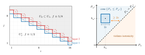
Both mechanisms are randomized isotonic adversaries whose posteriors factorize. Mechanism I needs a graded order with many large consecutive central rank levels: independent fair bits toggle the points of $K$ such levels across $K$ nested frontiers, every realization of the bits yields an isotonic function, and each probed point’s value depends on its own bit alone (Complete Isolation), so the game decouples into independent two-point Bernoulli tests. Mechanism II needs a separated core, an isotonic $b:\mathcal{P}\to[\tfrac{1}{3},\tfrac{2}{3}]$ that rises by at least $4\varepsilon$ across every strict relation: perturbing each value of $b$ independently by at most $\varepsilon$ keeps every realization inside the isotonic cone, the posterior factorizes across points, and the van Trees inequality (Gill and Levit, 1995) lower-bounds the estimation error at every query count. Planarity and MacMahon’s formula enter the sharp constants and the fast dynamic programs of Section 5, never the mechanisms themselves. Figure 1 shows both in their planar form.
3.2 The Main Theorem
On the grids $[m]^{d}$ the two mechanisms match the universal upper bound in every fixed dimension, across the loss class.
Theorem 2 (Main Theorem).
Fix an integer $d\geq 2\text{,}$ and let $\ell$ be a curved loss with parameters $(\eta,\beta,\alpha,\Lambda)$ or the entropic loss. For all integers $m\geq 2$ and $T\geq 1\text{,}$
| $$R_{T}^{*}\bigl([m]^{d},\ell\bigr)\;=\;\Theta\bigl(\min\bigl\{T,\;\Psi_{[m]^{d}}(T)\bigr\}\bigr),$$ |
with implied constants depending only on $d$ and the loss parameters.
The content of the theorem is geometric: the formula holds in every dimension through the same two mechanisms, and the entire loss dependence collapses into the constant, so the rate is governed by the entropy profile $H_{[m]^{d}}\text{.}$
Proof architecture.
The upper bound follows by evaluating Theorems 1 and 55 through Lemma 62. The two mechanisms run along the rank levels $A_{s}:=\{x\in[m]^{d}:\sum_{i}(x_{i}-1)=s\}\text{,}$ of which at least $m/2$ consecutive central ones carry at least $m^{d-1}/(2d)$ points apiece by the unimodality of $(|A_{s}|)_{s}\text{,}$ the only combinatorial input the grids require. Both price rounds through the posterior. A Mechanism I bit stays uncertain across the $\Theta(K^{2})$ rounds of its episode, its two candidate values differing by $\Theta(1/K)\text{,}$ so every informative round costs $\Omega(1/K^{2})\text{;}$ with $\Theta_{d}(m^{d-1}K)$ bits to resolve on $K\leq m/2$ of those levels, the ensemble yields $R_{T}^{*}([m]^{d})\gtrsim_{d}\min\{m^{d-1}K,\,T/K^{2}\}\text{,}$ and $T$ decides which branch of the minimum binds. Mechanism II perturbs the rank function itself, a separated core; each of the $m^{d}$ cells then receives $\Theta_{d}(T/m^{d})$ queries, and van Trees converts that query count into a per-cell estimation error, yielding $R_{T}^{*}([m]^{d})\geq\tfrac{3}{16}\,m^{d}\log\bigl(1+\tfrac{T}{540\,d^{2}m^{d+2}}\bigr)$ for $T\geq m^{d}\text{.}$ A curved loss enters the argument at exactly two points, the posterior-variance step of the bit ensemble and the regret-to-squared-error reduction of the separated core, where (1) substitutes the factor $\alpha\text{;}$ every other step concerns the Bernoulli observation law alone, and Pinsker’s inequality supplies $\alpha=2$ for the entropic loss. An elementary envelope comparison assembles these bounds into $\min\{T,\Psi_{[m]^{d}}(T)\}\text{.}$ Full proofs: Appendix K for the constructions and the merging, Appendix J for the loss substitutions; the planar squared-loss case carries the explicit constant $(1088\cdot 342)^{-1}$ through Appendix D.
In dimension one the grid is the chain, whose complete law is Theorem 46: at intermediate horizons the rate is $\Theta(T^{1/3}L_{T}^{2/3})$ with $L_{T}:=1+\log_{+}(n^{3}/T)$ and $\log_{+}x:=\max\{\log x,0\}\text{,}$ the logarithmic factor announced by the chain’s entropy in Section 2.2 and avoided in every dimension $d\geq 2$ (Appendix I).
3.3 The Three Phases and the Phase Criterion
Corollary 3 (Three-Phase Scaling Law).
Fix $d$ and $\ell$ as in Theorem 2. For all integers $m\geq 2$ and $T\geq 1\text{,}$
| $$R_{T}^{*}([m]^{d},\ell)\;=\;\begin{cases}\Theta_{d}(T),&T\lesssim_{d}m^{d-1}\quad\text{(Phase 0),}\\[2.0pt] \Theta_{d}\bigl(m^{2(d-1)/3}\,T^{1/3}\bigr),&m^{d-1}\lesssim_{d}T\lesssim_{d}m^{d+2}\quad\text{(Phase 1),}\\[2.0pt] \Theta_{d}\bigl(m^{d}\,\bigl[1+\log\tfrac{T}{m^{d+2}}\bigr]\bigr),&T\gtrsim_{d}m^{d+2}\quad\text{(Phase 2),}\end{cases}$$ | (3) |
with implied constants depending also on the loss parameters.
The optimization behind (3) is part of the proof of Theorem 2 in Appendix K. The phases have a physical reading: in Phase 0 the adversary lacks the budget to activate the combinatorial structure and every round costs $\Theta(1)\text{;}$ in Phase 1 a $K$-layer frontier balances its $\Theta_{d}(m^{d-1}K)$ bits against the observation cost $T/K^{2}$ at $K^{*}\asymp_{d}(T/m^{d-1})^{1/3}\text{;}$ in Phase 2 the $m^{d}$ cells decouple into independent scalar estimation problems and the regret turns logarithmic.
On the plane both the entropy and the envelope are exact. Order-preserving maps $[m]^{2}\to\{1,\ldots,K{+}1\}$ are in bijection with plane partitions in an $m\times m\times K$ box, and MacMahon’s formula counts them.
Theorem 4 (MacMahon’s Formula (MacMahon, 1916)).
For all integers $m,K\geq 1\text{,}$
| $$\Omega([m]^{2},K{+}1)\;=\;\prod_{i=1}^{m}\prod_{j=1}^{m}\frac{K+i+j-1}{i+j-1}.$$ | (4) |
Taking logarithms in (4) turns the count into a double sum, and an Euler–Maclaurin expansion of it gives the planar entropy law $H_{[m]^{2}}(K)=m^{2}\,\varphi(K/m)+O(\log m)\text{,}$ the error uniform in $K\text{,}$ with $\varphi(\alpha):=\int_{0}^{1}\!\!\int_{0}^{1}\log\bigl(1+\tfrac{\alpha}{s+t}\bigr)\,ds\,dt$ the Riemann limit of that sum (Lemma 14). The three-phase law sharpens accordingly, to $\Psi_{[m]^{2}}(T)=m^{2}\,\psi(T/m^{4})+O(m)$ as $T/m\to\infty$ with $\psi(c):=\inf_{\alpha>0}\{2\varphi(\alpha)+c/(4\alpha^{2})\}$ (Appendix C), and the Phase-1 constant lies between $7^{-7/3}\approx 0.0107$ and $\bigl(\tfrac{3\log 2}{4}\bigr)^{2/3}\approx 0.6465$ (Appendix M).
Which phases can occur is governed by the shape of $H_{\mathcal{P}}\text{.}$ Truncation at level $K$ splits an isotonic map valued in $\{0,\ldots,K{+}L\}$ injectively into one valued in $\{0,\ldots,K\}$ plus one valued in $\{0,\ldots,L\}\text{,}$ so $H_{\mathcal{P}}(K{+}L)\leq H_{\mathcal{P}}(K)+H_{\mathcal{P}}(L)\text{:}$ on every finite poset the entropy is subadditive, hence at most linear in $K\text{.}$ On a power-law window $H_{\mathcal{P}}(K)\asymp K^{\rho}$ this forces $\rho\leq 1\text{,}$ and balancing $K^{\rho}$ against $T/K^{2}$ caps the intermediate exponent of the envelope at $\rho/(\rho+2)\leq\tfrac{1}{3}\text{.}$ The regret never exceeds the envelope, so no finite poset sustains an intermediate phase with a larger exponent; the grid attains the cap in every dimension: extremal, not special. A linear regime of $H_{\mathcal{P}}$ produces the cube-root phase on every family characterized here, and entropy of the form $n\log(K{+}1)$ produces no intermediate phase at all. Posets of height at most two are of that kind: two antichains carry the whole order, any assignment on either extends isotonically, and the rate is $\Theta(n\log(1+T/n))\text{,}$ which Follow-the-Leader already attains under the squared loss. Fences, whose cover relations alternate in direction along a path, are among them (Proposition 67).
4 The Lipschitz Boundary
The universal upper bound rests on two prices: exp-concavity puts aggregation at $\tfrac{1}{\eta}H_{\mathcal{P}}(K)\text{,}$ and smoothness puts rounding at $\beta T/(8K^{2})\text{.}$ A kink degrades both at once: aggregation reverts to the $\sqrt{T\,H_{\mathcal{P}}(K)}$ of a generic bounded convex loss, and rounding turns linear in the resolution. Already on the one-point poset, where the comparator class is the interval $[0,1]\text{,}$ the squared loss has minimax regret $\Theta(\log T)\text{,}$ while under independent fair labels the absolute loss costs every prediction $\tfrac{1}{2}$ per round and lets the better endpoint recover half of $\lvert\sum_{t}(2y_{t}-1)\rvert$ in hindsight, forcing $\Theta(\sqrt{T})$ (Appendix J).
For $\tau\in(0,1)\text{,}$ the pinball loss $\ell_{\tau}(p,y):=\tau(y-p)_{+}+(1-\tau)(p-y)_{+}$ is the loss of quantile estimation, with $\rho_{\tau}:=\tau(1-\tau)\text{;}$ the absolute loss is $2\ell_{1/2}\text{.}$ On grids the rate is a square-root law, uniform in the quantile:
| $$R_{T}^{*}\bigl([m]^{d},\ell_{\tau}\bigr)\;=\;\Theta_{d}\Bigl(\min\bigl\{\rho_{\tau}T,\;\sqrt{\rho_{\tau}\,m^{d-1}\,T}\bigr\}\Bigr),\quad R_{T}^{*}\bigl([m]^{d},\lvert\cdot\rvert\bigr)\;=\;\Theta_{d}\bigl(\min\{T,\sqrt{m^{d-1}T}\}\bigr)$$ |
(Theorem 56, proved in Appendix J). The upper bound aggregates the $e^{H_{[m]^{d}}(1)}$ indicators of upsets, the upward-closed subsets of the grid, under exponential weights: the layer-cake identity $f=\int_{0}^{1}\mathbf{1}\!\left[\cdot\in\{f\geq s\}\right]\,ds$ reduces the linearized regret against $\mathcal{F}_{\mathcal{P}}^{\uparrow}$ to the regret against a single upset, and a small-loss bound, its benchmark $\rho_{\tau}T$ witnessed by the empty and full upsets, yields the rate. The lower bound draws $\mathrm{Ber}(1-\tau)$ labels on one central rank level, where the pinball Bayes risk is flat at $\rho_{\tau}\text{,}$ fair coins at $\tau=\tfrac{1}{2}\text{:}$ the learner pays $\rho_{\tau}$ each round, while the comparator picks the better endpoint at each of the $\Theta_{d}(m^{d-1})$ antichain points independently and collects their binomial fluctuations.
No resolution enters either bound; the grid disappears from the analysis, the upper bound retaining only $H_{[m]^{d}}(1)$ and the lower bound only the size of one rank level. On the plane, $\sqrt{mT}$ is exactly what the single-scale bound of Appendix L yields at coarse scales, now met without slack: what stationarity and smoothness together recover for curved losses is what the kink forfeits. The square-root rate is attained efficiently: the grid splits into planes at no cost in entropy, and on the queried one the exponential-weights prediction is a single weighted upset marginal, one call per round to the $O(m^{2})$ dynamic program of Lemma 38 (Appendix J).
5 Polynomial-Time Algorithms
Realizing Theorem 1 directly means maintaining $e^{H_{\mathcal{P}}(K)}$ experts, exponential in $m^{d-1}$ on grids. This section removes the obstacle: its endpoint is Theorem 7, a horizon-free polynomial-time learner rate-optimal on $[m]^{d}$ for every fixed $d$ and every loss of the Theorem 2 family. The route runs through the plane: two complementary engines, their lower envelope made horizon-free by a rate-doubling wrapper, and a slicing step that lifts the planar learner to every dimension.
5.1 Column-Independent Chain Exponential Weights
The first engine drops the constraints between columns: each column $i\in[m]$ is treated as an independent chain, carrying its own exponential weights over the $\binom{m+K}{K}$ non-decreasing $G_{K}$-valued functions $\mathcal{F}_{[m],K}^{\uparrow}\text{.}$ Because the squared loss is row-additive, the per-column weight factorizes across rows, and the predictive mean at a query $x_{t}=(i_{t},j_{t})$ reduces to a $(K{+}1)$-state forward-backward dynamic program along the chain, $O(mK)$ per round, only the queried column updating.
Every $f\in\mathcal{F}_{[m]^{2}}^{\uparrow}$ restricts column-wise to a non-decreasing function, so $\mathcal{F}_{[m]^{2}}^{\uparrow}\subseteq\prod_{i=1}^{m}\mathcal{F}_{[m]}^{\uparrow}\text{;}$ enlarging the comparator class cannot decrease the regret, which then splits as $R_{T}\leq\sum_{i=1}^{m}R_{i}\text{.}$ Per column, the chain case of Theorem 1 gives $R_{i}\leq 2\log\binom{m+K}{K}+T_{i}/(4K^{2})$ with $T_{i}:=|\{t:i_{t}=i\}|\text{,}$ and $\sum_{i}T_{i}=T\text{,}$ so $R_{T}\leq 2m\log\binom{m+K}{K}+T/(4K^{2})\text{.}$ At a level attaining the infimum, and with $R_{T}\leq T\text{,}$ this gives $R_{T}\leq\min\{T,\Psi_{\mathrm{col}}(T)\}$ with $\Psi_{\mathrm{col}}(T):=\inf_{K\in\mathbb{N}_{+}}\bigl\{2m\,\log\binom{m+K}{K}+T/(4K^{2})\bigr\}$ (Theorem 35, proved in Section F.1).
In Phase 2 ($T\gg m^{4}$), $K^{*}=\Theta(\sqrt{T}/m)$ gives $\Psi_{\mathrm{col}}(T)=\Theta(m^{2}\log(T/m^{4}))\text{,}$ matching Corollary 3 at the $\Theta$ level. In Phase 1 the engine pays for the enlargement: for $m\log m\lesssim T\lesssim m^{4}\text{,}$ $\Psi_{\mathrm{col}}(T)=\Theta(m^{2/3}\,T^{1/3}\,[1+\log(m^{4}/T)]^{2/3})\text{,}$ the factor above the minimax rate being of order $(\log m)^{2/3}$ through the bulk of the phase and fading only at its far end. The factor has an algebraic source: dropping the inter-column constraints inflates the entropy from $2H_{[m]^{2}}(K)=\Theta(mK)$ to $2m\log\binom{m+K}{K}=\Theta(mK[1+\log(m/K)])$ for $K\leq m\text{,}$ and the logarithm is not negligible at $K^{*}\ll m\text{.}$ Widening columns to strips does not help: every regret bound the standard exp-concave EW analysis produces for a strip decomposition retains the factor (Theorem 44); closing it takes a different decomposition.
5.2 Surrogate Threshold-Indexed Exponential Weights
Decomposing by threshold layer instead closes the gap. The engine has three parts: a Gibbs identity that factorizes the exponential weights across layers once the latent representation is enlarged, a surrogate loss that dominates the true loss on the enlarged representation and is tight on its nested part, and an $O(m^{2})$ dynamic program for upset marginals.
Gibbs layering.
For $h:[m]^{2}\to\{0,1,\ldots,K\}$ and $u\in[m]^{2}\text{,}$ $h(u)=\sum_{r}\mathbf{1}\!\left[h(u)\geq r\right]$ and $h(u)^{2}=\sum_{r}(2r-1)\,\mathbf{1}\!\left[h(u)\geq r\right]\text{,}$ the first identity writing $h$ as the count of thresholds it exceeds, the second following from the first via $\sum_{r=1}^{k}(2r-1)=k^{2}\text{.}$ Substituted into the exponential weight $\exp(-\tfrac{1}{2}\sum_{s<t}(g(x_{s})-y_{s})^{2})$ of a grid function $g=h/K\text{,}$ they factorize the weight into per-layer, per-cell factors indexed by the threshold upsets $U_{r}(h):=\{h\geq r\}\text{;}$ once the nesting constraint on the tuple $(U_{1},\ldots,U_{K})$ is dropped, the factorization is complete and the weights update layer by layer. In the other direction, for $z_{1},\ldots,z_{K}\in\{0,1\}$ with $k:=\sum_{r}z_{r}\text{,}$ the strictly increasing coefficients give $\sum_{r}(2r-1)\,z_{r}\geq k^{2}\text{,}$ with equality exactly when $(z_{1},\ldots,z_{K})$ is the prefix of length $k\text{:}$ the inequality that makes the relaxation free.
Generalized experts and the surrogate.
A generalized expert is an arbitrary tuple $G=(U_{1},\ldots,U_{K})\in\mathcal{U}^{K}$ of upsets of $[m]^{2}\text{,}$ predicting $g_{G}(x):=\tfrac{1}{K}\sum_{r}\mathbf{1}\!\left[x\in U_{r}\right]\text{;}$ there are $\binom{2m}{m}^{K}$ of them, the upsets being in bijection with monotone lattice paths, $|\mathcal{U}|=\binom{2m}{m}\text{,}$ and every $g_{G}$ is isotonic, a nonnegative combination of upset indicators, as is every average of them. Under the squared loss the surrogate charges $G$ the loss increments of its layers, additive across layers by construction,
| $$\widetilde{\ell}(G;\,x,y)\;:=\;y^{2}\,+\,\sum_{r=1}^{K}\!\left(\frac{2r-1}{K^{2}}-\frac{2y}{K}\right)\mathbf{1}\!\left[x\in U_{r}\right],$$ | (5) |
with per-layer coefficient $c_{r,t}:=(2r-1)/K^{2}-2y_{t}/K$ at round $t\text{,}$ and we abbreviate $\widetilde{\ell}_{t}(G):=\widetilde{\ell}(G;\,x_{t},y_{t})\text{.}$
The surrogate dominates the true loss, $\widetilde{\ell}(G;\,x,y)\geq(g_{G}(x)-y)^{2}\text{,}$ with equality exactly when the membership vector $(\mathbf{1}\!\left[x\in U_{1}\right],\ldots,\mathbf{1}\!\left[x\in U_{K}\right])$ is a prefix of ones, hence at every $x$ once $U_{1}\supseteq\cdots\supseteq U_{K}$ (Lemma 37); in the loss-increment form this is a rearrangement bound valid for every convex loss (Lemma 57), and that form is what carries the engine across the loss class in Section 5.4. Each layer’s marginal $\Pr_{U\sim\mu}[x\in U]$ under $\mu(U)\propto\prod_{u\in U}w_{u}$ is computable in $O(m^{2})$ time by parametrizing upsets through their frontiers and running a forward-backward program over cutoffs (Lemma 38). Algorithm 2 keeps one weight per cell in each layer, so that the global measure is the product $\pi_{t}$ of the $K$ layer measures, runs that program once in each layer, and predicts the average of the $K$ marginals; Section F.2 proves all three.
Theorem 5 (Surrogate Upper Bound).
Fix any integers $m\geq 2$ and $K\in\mathbb{N}_{+}\text{.}$ Algorithm 2 runs in per-round time $O(Km^{2})$ and, for any sequence $(x_{t},y_{t})_{t=1}^{T}\in[m]^{2}\times[0,1]\text{,}$ satisfies $R_{T}\leq 2K\,\log\!\binom{2m}{m}+T/(4K^{2})\text{.}$ At a level attaining the infimum below, and with $R_{T}\leq T\text{,}$
| $$R_{T}\;\leq\;\min\!\bigl\{T,\;\Psi_{\mathrm{surr}}(T)\bigr\},\quad\Psi_{\mathrm{surr}}(T)\;:=\;\inf_{K\in\mathbb{N}_{+}}\!\biggl\{2K\,\log\!\binom{2m}{m}\,+\,\frac{T}{4K^{2}}\biggr\}.$$ | (6) |
By Stirling’s formula, $\log\binom{2m}{m}=2m\log 2-O(\log m)\text{,}$ so $K^{*}=\Theta((T/m)^{1/3})$ and $\Psi_{\mathrm{surr}}(T)=\Theta(m^{2/3}T^{1/3})\text{:}$ rate-optimal throughout Phase 1, with no logarithmic factor. In Phase 2 the envelope stays at $T^{1/3}$ while the rate turns logarithmic, so the two engines are complementary.
5.3 Combined Strategy and Horizon-Free Wrapper
For a known horizon the better engine can be chosen in advance: with $\Phi(T):=\min\{T,\Psi_{\mathrm{col}}(T),\Psi_{\mathrm{surr}}(T)\}\text{,}$ running whichever of Algorithm 1 and Algorithm 2 has the smaller envelope, at its optimizing level, takes $\mathrm{poly}(m,T)$ per round and satisfies $R_{T}\leq\Phi(T)$ (Theorem 40), the trivial bound $R_{T}\leq T$ holding for any predictions in $[0,1]\text{.}$
Evaluating the three terms phase by phase,
| $$\Phi(T)\;=\;\begin{cases}\Theta(T),&T\lesssim m,\\ \Theta(m^{2/3}T^{1/3}),&m\lesssim T\lesssim m^{4},\\ \Theta(m^{2}\log(T/m^{4})),&T\gg m^{4},\end{cases}$$ | (7) |
matching Theorem 2 at the $\Theta$ level at every horizon.
Rate-doubling wrapper.
Theorem 40 requires advance knowledge of $T\text{.}$ Partition the time axis into epochs $k=1,2,\ldots$ of adaptive length
| $$L_{k}\;:=\;\max\!\bigl\{L\in\mathbb{N}_{+}:\Phi(L)\leq 2^{k-1}\bigr\},$$ | (8) |
so the regret of a horizon-$L_{k}$ instance of the combined strategy within epoch $k$ is $\leq\Phi(L_{k})\leq 2^{k-1}\text{,}$ summing geometrically. Different epochs use freshly initialized algorithms (no shared state); see Algorithm 3 in Section F.3.
Theorem 6 (Horizon-Free Polynomial-Time Rate-Optimal Algorithm).
Algorithm 3 runs in $\mathrm{poly}(m,t)$ per-round time at every round $t\geq 1$ and, for any $T\geq 1$ and any sequence $(x_{t},y_{t})_{t=1}^{T}\in[m]^{2}\times[0,1]\text{,}$ satisfies $R_{T}\leq 4\,\Phi(T)+2\text{.}$
5.4 Every Fixed Dimension, Every Loss
The planar learner lifts to every dimension by slicing. Write each $x\in[m]^{d}$ as $(z,i,j)$ with $z\in[m]^{d-2}\text{:}$ the slices $\{z\}\times[m]^{2}$ partition the grid into $m^{d-2}$ copies of the plane, and the learner runs an independent planar instance on each, advancing only the queried one.
Theorem 7 (Slicing).
Fix an integer $d\geq 2$ and let $\ell$ be a loss of the Theorem 2 family. There is a horizon-free deterministic learner for $[m]^{d}$ with $\mathrm{poly}(m,t)$ per-round time achieving, for all integers $m\geq 2$ and $T\geq 1$ and every sequence,
| $$R_{T}\;\leq\;C_{d,\ell}\,\min\bigl\{T,\;\Psi_{[m]^{d}}(T)\bigr\},$$ |
with $C_{d,\ell}$ depending only on $d$ and the loss parameters.
A global comparator restricts isotonically to every slice, so the benchmark only tightens slicewise and regret adds across slices; Jensen’s inequality then recombines the per-slice bounds through the concave three-phase majorant of (7), reproducing the three phases of Corollary 3 exactly (Appendix K). Behind the recombination is an entropy accounting: $m^{d-2}$ planar slices at $\Theta(mK)$ apiece reproduce the global $\Theta_{d}(m^{d-1}K)\text{,}$ while slicing into chains would inflate each factor by the logarithm behind the strip barrier of Theorem 44; the plane is the smallest unit on which slicing is free. For losses beyond the squared one, Appendix J rebuilds the planar engine: the loss-increment surrogate keeps the layer factorization and the upset dynamic program, stationarity and the arcsine grid price the rounding, and the wrapper framework carries over with rescaled constants (Proposition 58).
The costs are explicit. At level $K\text{,}$ Algorithm 1 runs in $O(mK)$ time and $O(m^{2}K)$ storage per round and Algorithm 2 in $O(Km^{2})$ time and storage; at the rate-optimal levels this is $O(m^{5/3}T^{1/3})$ per round in Phase 1 and $O(\sqrt{T})$ per round with $O(m\sqrt{T})$ storage in Phase 2. These figures are for the planar engines; the sliced learner advances only the queried slice and stores state for the touched ones. Measured, Algorithm 2 at $m=24\text{,}$ $K=6$ takes $1.3$ ms per round in unoptimized single-core Python, $35$ seconds for the calibration stream of Appendix A, where synthetic runs locate the transition at $T\asymp m^{4}$ and the crossover between the two engines.
6 Discussion
On every grid $[m]^{d}$ with $d\geq 2$ fixed, the minimax regret of online isotonic regression is $\Theta(\min\{T,\Psi_{[m]^{d}}(T)\})$ for every loss of the Theorem 2 family, and a horizon-free polynomial-time learner attains the rate (Theorem 7): this settles, on these grids, the problem posed by Kotłowski et al. (2017). The boundary cases have their own laws: the square-root rate of Theorem 56 for the pinball family, and the complete chain law of Theorem 46 in dimension one.
Our protocol allows repeated queries. Every upper bound is pathwise, so the algorithms and their guarantees hold verbatim under distinct queries, in particular under the random-permutation model of Kotłowski et al. (2017). Distinct queries reshape the minimax question itself: they force $T\leq m^{d}\text{,}$ so Phase 2, which begins at $T\gtrsim_{d}m^{d+2}\text{,}$ cannot even be posed; through $T\lesssim_{d}m^{d-1}$ the two protocols share the rate $\Theta_{d}(T)\text{,}$ since fair-coin labels on a central rank level, an antichain of $\Theta_{d}(m^{d-1})$ points, cost any learner at least $\tfrac{1}{4}$ per round in expectation while some isotonic function fits them exactly; and on the remaining window $m^{d-1}\lesssim_{d}T\leq m^{d}$ the sharp rate is open, between the $\Omega_{d}(m^{d-1})$ of the same construction and the pathwise $O_{d}(m^{2(d-1)/3}T^{1/3})\text{.}$
We conjecture that $R_{T}^{*}(\mathcal{P})=\Theta(\min\{T,\Psi_{\mathcal{P}}(T)\})$ for every finite $\mathcal{P}\text{,}$ matching Theorem 1. The open problem is to establish the conjecture, and to match it in polynomial time, on every finite poset; Follow-the-Leader is the current baseline (Theorem 45).
References
- Contributions to the theory of the Barnes function. International Journal of Mathematics and Computer Science 9 (1), pp. 11–30. Note: arXiv preprint math/0308086 (2003) Cited by: Fact 12.
- Surrogate regret bounds for bipartite ranking via strongly proper losses. Journal of Machine Learning Research 15, pp. 1653–1674. Cited by: §2.1.
- The theory of the G-function. Quarterly Journal of Pure and Applied Mathematics 31, pp. 264–314. Cited by: Fact 12.
- Adult. Note: UCI Machine Learning RepositoryDOI: 10.24432/C5XW20 Cited by: §A.2.
- Classifier calibration with ROC-regularized isotonic regression. In Proceedings of the 27th International Conference on Artificial Intelligence and Statistics (AISTATS), Proceedings of Machine Learning Research, Vol. 238, pp. 1972–1980. Cited by: §1.
- Convex optimization. Cambridge University Press, Cambridge. External Links: ISBN 9780521833783 Cited by: Appendix H, Fact 9.
- Prediction, learning, and games. Cambridge University Press. External Links: ISBN 9780521841085, Document Cited by: §J.5, §F.1.3, Appendix H, §1, §2.1.
- On matrix estimation under monotonicity constraints. Bernoulli 24 (2), pp. 1072–1100. External Links: Document Cited by: §1.
- Designs for single- or multiple-agent phase I trials. Biometrics 60 (3), pp. 661–669. External Links: Document Cited by: §1.
- A chaining algorithm for online nonparametric regression. In Proceedings of the 28th Conference on Learning Theory (COLT), Proceedings of Machine Learning Research, Vol. 40, pp. 764–796. Cited by: §L.3, §1.
- Applications of the van Trees inequality: a Bayesian Cramér–Rao bound. Bernoulli 1 (1–2), pp. 59–79. External Links: Document Cited by: §1, §3.1, Fact 30.
- Online isotonic regression. In Proceedings of the 29th Conference on Learning Theory (COLT), Proceedings of Machine Learning Research, Vol. 49, pp. 1165–1189. Cited by: §J.4, §J.5, §L.1, §1, §1, §2.3, §2.3.
- Random permutation online isotonic regression. In Advances in Neural Information Processing Systems 30 (NIPS 2017), I. Guyon, U. von Luxburg, S. Bengio, H. M. Wallach, R. Fergus, S. V. N. Vishwanathan, and R. Garnett (Eds.), pp. 4180–4189. Cited by: §1, §1, §6, §6.
- Minimax adaptive online nonparametric regression over Besov spaces. In Advances in Neural Information Processing Systems 38 (NeurIPS), Cited by: §L.5, §L.6, §1.
- Minimax-optimal and locally-adaptive online nonparametric regression. In Proceedings of the 36th International Conference on Algorithmic Learning Theory (ALT), Proceedings of Machine Learning Research, Vol. 272. Cited by: §L.5, §L.6, §1.
- Combinatory analysis. Vol. 2, Cambridge University Press, Cambridge. Cited by: §K.5, §1, Theorem 4.
- Error bounds and exponential improvement for the asymptotic expansion of the Barnes $G$-function. Proceedings of the Royal Society A 470 (2172), pp. 20140534. External Links: Document Cited by: §C.5.
- Predicting good probabilities with supervised learning. In Proceedings of the 22nd International Conference on Machine Learning (ICML), Bonn, Germany, pp. 625–632. External Links: Document Cited by: §1.
- NIST Digital Library of Mathematical Functions. Note: https://dlmf.nist.gov/, Release 1.2.7 of 2026-06-15 Cited by: §C.5.
- Online non-parametric regression. In Proceedings of the 27th Conference on Learning Theory (COLT), Proceedings of Machine Learning Research, Vol. 35, pp. 1232–1264. Cited by: §L.2, §L.4, §L.4, §1, §2.2, §3.1.
- A chromatic-like polynomial for ordered sets. In Proceedings of the Second Chapel Hill Conference on Combinatorial Mathematics and Its Applications, Chapel Hill, NC, pp. 421–427. Cited by: §1, §2.2.
- Introduction to nonparametric estimation. Springer Series in Statistics, Springer, New York. External Links: ISBN 9780387790510, Document Cited by: §J.3, §J.4, §K.1, §E.1.5.
- A game of prediction with expert advice. Journal of Computer and System Sciences 56 (2), pp. 153–173. External Links: Document Cited by: §M.1, §1.
- Continual reassessment method for partial ordering. Biometrics 67 (4), pp. 1555–1563. External Links: Document Cited by: §1.
- Probabilistic computations: toward a unified measure of complexity. In 18th Annual Symposium on Foundations of Computer Science (FOCS), Providence, RI, USA, pp. 222–227. External Links: Document Cited by: §E.1, §E.2, §2.1.
- Transforming classifier scores into accurate multiclass probability estimates. In Proceedings of the Eighth ACM SIGKDD International Conference on Knowledge Discovery and Data Mining (KDD), Edmonton, Alberta, Canada, pp. 694–699. External Links: Document Cited by: §1.
Appendix A Experiments
We run the learners of Section 5 on synthetic streams and on a real calibration task.
A.1 Synthetic Streams
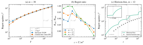
Figure 3 reports the synthetic runs, every known-horizon engine at the level minimizing its bound for that horizon; the dynamic programs behind them agree with brute-force enumeration of their expert classes to within $10^{-13}$ on eight small $(m,K)$ pairs (Section A.3). At $m=30$ both engines follow the $T^{1/3}$ reference until $T\approx m^{4}\text{;}$ beyond the transition Algorithm 1 bends onto the logarithmic rate of Theorem 35, while Algorithm 2 stays on the cube-root envelope of (6). The paired ratio of panel (b) locates the crossover directly: near one before the transition and falling beyond it, to $0.77$ at $m=18$ and $c=T/m^{4}=10\text{.}$ Panel (c) resolves the horizon-free wrapper at $m=12\text{,}$ the rate-doubling restarts visible as steps and the full path within a factor of three of fresh known-horizon runs, consistent with the factor four of Theorem 6. The streams are benign, and the exponents owe nothing to adversarial labels: every upper bound is pathwise, an i.i.d. stream is among the covered sequences, and the labels inside both lower-bound constructions are themselves Bernoulli.
A.2 Real-Data Calibration
The calibration experiment asks whether the two-dimensional monotone structure earns its keep on real data. A logistic model is trained on 40 percent of UCI Adult [Becker and Kohavi, 1996], its incomplete rows discarded, with education withheld from its features, so the covariate keeps signal the model does not use; the remaining $T=27{,}134$ examples stream under squared loss on the $16\times 16$ grid formed by 16 model-score quantiles and the 16 ordinal education levels, with Algorithm 2 at the discretization level minimizing (6). Margins are paired, mean $\pm$ one standard error over twenty splits and stream orders. Algorithm 2 pays $2{,}975.0\pm 5.8$ in cumulative squared loss, beating the score-only calibrator (online isotonic regression on the score axis alone, the chain case of the problem) by $52.0\pm 2.8\text{,}$ and a per-cell smoothed running mean on the same grid by $31.9\pm 1.0\text{,}$ each on 20 of 20 splits; a global running mean, using neither feature, pays $5{,}057.8\text{.}$
Both ingredients carry their weight: beating the score-only calibrator shows the covariate is used, and beating the per-cell mean, which sees the same two features, shows the order constraint doing work of its own. The constraint is worth more as the cells thin, and on the finest of three grids the per-cell mean has fallen behind the score-only calibrator while Algorithm 2 leads both: refining the grid pays only when the order constraint is exploited. The tradeoff behind the phases is visible along the horizon. With the learners tuned to each horizon, the margin over the score-only calibrator runs $-16.0\text{,}$ $-11.3\text{,}$ $-0.2\text{,}$ $+52.0$ at $T=2{,}713\text{,}$ $6{,}783\text{,}$ $13{,}567\text{,}$ $27{,}134\text{:}$ the richer comparator class pays for its entropy first and collects afterwards, a crossover between two comparator classes.
Two controls pin the reading down. Shuffling the covariate within the stream destroys its signal and touches nothing else: the $+52.0$ margin flips to $-133.6\text{,}$ all twenty splits lost, so the gain is the signal. Replacing the logistic base model with gradient boosting shrinks the residual signal in the covariate, and the margin drops to $15.4\pm 2.3\text{,}$ still 19 of 20, while the margin over the per-cell mean holds at $26.6\pm 0.7$ on 20 of 20: the effect survives a stronger base model. On the $24\times 16$ grid even the horizon-free wrapper beats both baselines on 20 of 20 splits ($28.6\pm 3.1$ and $57.5\pm 1.3$), restart overhead included; on the $16\times 16$ grid that overhead measures about three percent of cumulative loss. Every margin in this paragraph is six standard errors or more.
Grid resolution.
Refining the score axis thins the cells and raises the value of the order constraint. Against the per-cell smoothed running mean the margin of Algorithm 2 runs $+2.0\pm 0.7\text{,}$ $+31.9\pm 1.0\text{,}$ $+125.0\pm 1.0$ as the score axis refines from 12 to 16 to 24 quantiles (education pooled to 12 levels in the first case; the last is a $24\times 16$ grid), with roughly $188\text{,}$ $106\text{,}$ and $71$ observations per cell. The protocol is otherwise as above, with twenty splits and stream orders per configuration.
A.3 Correctness of the Dynamic Programs
We verify the DP implementations from Section 5 by directly comparing per-round predictions against brute-force enumeration. For Surrogate TI-EW, the brute force enumerates all $K$-tuples of upsets on $[m]^{2}$ ($\binom{2m}{m}^{K}$ generalized experts). For Column-Indep. Chain EW, the brute force maintains an independent exponential-weight measure on each column over the $\binom{m+K}{K}$ non-decreasing $K$-grid functions—equivalent to exponential weights over $\binom{m+K}{K}^{m}$ column-independent experts on $[m]^{2}\text{.}$ Both use standard exponential weights with $\eta=1/2$—surrogate loss for the former, squared loss for the latter.
The setup follows Section A.1: Bernoulli labels with mean $f^{*}(i,j)=0.25+(i+j-2)/[4(m-1)]$ on $[m]^{2}\text{,}$ i.i.d. uniform queries, $T=200$ rounds, seed $=42\text{.}$ At each round $t\text{,}$ we compute the discrepancy $|\hat{y}_{t}^{\mathrm{DP}}-\hat{y}_{t}^{\mathrm{BF}}|$ between the DP and brute-force predictions.
Table 1 reports $\max_{t}|\hat{y}_{t}^{\mathrm{DP}}-\hat{y}_{t}^{\mathrm{BF}}|$ for $8$ $(m,K)$ configurations. All values are $\leq 10^{-13}\text{;}$ the DP and brute-force predictions agree within machine precision.
| $m$ | $K$ | Surr. max disc | Col. max disc |
|---|---|---|---|
| 3 | 2 | $1.33\times 10^{-15}$ | $9.99\times 10^{-16}$ |
| 3 | 3 | $1.72\times 10^{-15}$ | $1.22\times 10^{-15}$ |
| 3 | 4 | $1.33\times 10^{-15}$ | $1.22\times 10^{-15}$ |
| 4 | 2 | $2.28\times 10^{-15}$ | $6.66\times 10^{-16}$ |
| 4 | 3 | $1.89\times 10^{-15}$ | $9.99\times 10^{-16}$ |
| 5 | 2 | $2.00\times 10^{-15}$ | $6.66\times 10^{-16}$ |
| 5 | 3 | $5.35\times 10^{-14}$ | $7.77\times 10^{-16}$ |
| 6 | 2 | $2.67\times 10^{-15}$ | $8.88\times 10^{-16}$ |
Code availability.
The complete implementation of the three algorithms, the brute-force verification harness, the calibration experiment, and the figure-generation scripts are available at https://github.com/sichen-wang/Online-Isotonic-Regression_Code.
Appendix B Block Residual Property
This appendix provides the complete proof of Lemma 8. The argument proceeds in four steps: (i) a $[0,1]$-projection shows that the box-constrained and unconstrained isotonic least-squares problems share the same minimum, reducing the lemma to a statement about minimizers of the relaxed problem; (ii) a strictly feasible point built from a linear extension certifies Slater’s condition; (iii) the standard KKT theorem then yields stationarity and complementary slackness in explicit form; and (iv) summing the KKT stationarity equation over the complete level set $C_{c}$ of $f^{*}$ (which contains unqueried elements as well), interior dual multipliers cancel pairwise, boundary edges vanish by complementary slackness, and unqueried elements contribute zero (since $w_{u}=0$), yielding the Block Residual identity. The key observation is in step (iv): the summation must extend over the complete level set $C_{c}$ rather than over the queried subset $B_{c}$ alone, so that all complementary slackness relations on boundary edges are activated.
Recall.
We use the following notation. Let $\mathcal{F}_{\mathcal{P}}^{\uparrow}$ denote the class of $[0,1]$-valued order-preserving (isotonic) maps on a finite poset $(\mathcal{P},\preceq)$ with $n:=|\mathcal{P}|\text{.}$ Given a sequence $(x_{t},y_{t})_{t=1}^{T}\in\mathcal{P}\times[0,1]\text{,}$ let $w_{u}:=|\{t:x_{t}=u\}|$ denote the query count, set $s_{u}:=\sum_{t\,:\,x_{t}=u}y_{t}$ and $\bar{y}_{u}:=s_{u}/w_{u}$ (defined only for $w_{u}>0$); let $f^{*}\in\operatorname*{arg\,min}_{f\in\mathcal{F}_{\mathcal{P}}^{\uparrow}}\sum_{t=1}^{T}(f(x_{t})-y_{t})^{2}$ denote the constrained least-squares solution; let $B_{c}:=\{u\in\mathcal{P}:w_{u}>0,\,f^{*}(u)=c\}$ be the set of queried elements assigned value $c\text{;}$ and let $C_{c}:=\{u\in\mathcal{P}:f^{*}(u)=c\}$ be the corresponding complete level set, which includes unqueried elements (those with $w_{u}=0$). Thus $C_{c}\supseteq B_{c}\text{.}$
Lemma 8 (Block Residual).
Let $(\mathcal{P},\preceq)$ be a finite poset. Given any sequence $(x_{t},y_{t})_{t=1}^{T}\in\mathcal{P}\times[0,1]\text{,}$ let $f^{*}\in\operatorname*{arg\,min}_{f\in\mathcal{F}_{\mathcal{P}}^{\uparrow}}\sum_{t=1}^{T}(f(x_{t})-y_{t})^{2}\text{;}$ $w_{u}:=|\{t:x_{t}=u\}|\text{;}$ $\bar{y}_{u}:=w_{u}^{-1}\sum_{t:x_{t}=u}y_{t}$ (for $w_{u}>0$); and $B_{c}:=\{u\in\mathcal{P}:w_{u}>0,\,f^{*}(u)=c\}$ for each value $c$ attained by $f^{*}\text{.}$ Then $\sum_{u\in B_{c}}w_{u}(c-\bar{y}_{u})=0\text{,}$ equivalently, $\sum_{t\,:\,x_{t}\in B_{c}}(f^{*}(x_{t})-y_{t})=0\text{.}$
Proof.
Step 1 (Box-constraint reduction). Define the Euclidean projection $\Pi:\mathbb{R}\to[0,1]$ by $\Pi(z):=\min\{1,\max\{0,z\}\}\text{.}$ Since $\Pi$ is non-decreasing, isotonicity is preserved: if $\tilde{f}:\mathcal{P}\to\mathbb{R}$ is order-preserving, then $\Pi\circ\tilde{f}\in\mathcal{F}_{\mathcal{P}}^{\uparrow}\text{.}$ For any $y\in[0,1]$ and any $z\in\mathbb{R}\text{,}$
| $$(\Pi(z)-y)^{2}\;\leq\;(z-y)^{2},$$ | (9) |
by direct case analysis on $z\text{:}$ equality holds for $z\in[0,1]\text{;}$ the inequality is immediate from $y\leq 1<z$ when $z>1\text{,}$ and follows by symmetry when $z<0\text{.}$
Let $\mathcal{F}_{\mathcal{P}}^{\mathbb{R}}:=\{\tilde{f}:\mathcal{P}\to\mathbb{R}\mid u\preceq v\,\Rightarrow\,\tilde{f}(u)\leq\tilde{f}(v)\}$ denote the class of real-valued order-preserving functions (without the box constraint), and consider the relaxed problem $\min_{\tilde{f}\in\mathcal{F}_{\mathcal{P}}^{\mathbb{R}}}\sum_{t}(\tilde{f}(x_{t})-y_{t})^{2}\text{.}$ Any minimizer $\tilde{f}^{*}$ of the relaxed problem satisfies $\Pi\circ\tilde{f}^{*}\in\mathcal{F}_{\mathcal{P}}^{\uparrow}\text{,}$ and by (9) together with $y_{t}\in[0,1]\text{,}$
| $$\sum_{t}\bigl(\Pi(\tilde{f}^{*}(x_{t}))-y_{t}\bigr)^{2}\;\leq\;\sum_{t}\bigl(\tilde{f}^{*}(x_{t})-y_{t}\bigr)^{2}.$$ |
Hence the minimum over $\mathcal{F}_{\mathcal{P}}^{\uparrow}$ is no larger than that over $\mathcal{F}_{\mathcal{P}}^{\mathbb{R}}\text{;}$ the reverse inequality follows from $\mathcal{F}_{\mathcal{P}}^{\uparrow}\subseteq\mathcal{F}_{\mathcal{P}}^{\mathbb{R}}\text{,}$ so the two problems share the same minimum. Consequently, the $f^{*}$ in the lemma statement (whose loss equals this common minimum and which lies in $\mathcal{F}_{\mathcal{P}}^{\mathbb{R}}$) is also a minimizer of the relaxed problem.
The KKT analysis below is therefore applied to the relaxed problem; the Block Residual identity, being a statement about $f^{*}$ itself, transfers back to the original (box-constrained) setting once established for the relaxation.
Step 2 (Convex program formulation). Expanding the squared sum and dropping the $f$-independent constant $\sum_{t}y_{t}^{2}\text{,}$
| $$\sum_{t=1}^{T}(f(x_{t})-y_{t})^{2}\;=\;\widetilde{\Phi}(f)\,+\,\sum_{t=1}^{T}y_{t}^{2},\qquad\widetilde{\Phi}(f)\;:=\;\sum_{u\in\mathcal{P}}\bigl(w_{u}f(u)^{2}-2s_{u}f(u)\bigr).$$ |
The relaxed problem is therefore equivalent to
| $$\min_{f\in\mathbb{R}^{\mathcal{P}}}\widetilde{\Phi}(f)\qquad\text{subject to}\qquad f(u)\leq f(v)\;\;\text{for all }u\prec v.$$ |
Let $E:=\{(u,v)\in\mathcal{P}^{2}:u\prec v\}\text{;}$ using all strict pairs (rather than only Hasse-diagram edges) does not affect the minimizer or the structure of the KKT analysis below. The constraint functions $g_{u,v}(f):=f(u)-f(v)\leq 0\text{,}$ $(u,v)\in E\text{,}$ are affine. Both $\widetilde{\Phi}$ and the $g_{u,v}$ are convex and differentiable.
Step 3 (Slater’s condition and KKT). Let $\tau:\mathcal{P}\to\{1,\ldots,n\}$ be any linear extension of $\mathcal{P}$ (existence guaranteed by the Szpilrajn extension theorem). Setting $f_{0}(u):=\tau(u)\text{,}$ every constraint becomes strict: for each $(u,v)\in E\text{,}$
| $$g_{u,v}(f_{0})\;=\;\tau(u)-\tau(v)\;\leq\;-1\;<\;0.$$ |
Hence Slater’s condition is satisfied.
Fact 9 (KKT for affine convex programs under Slater’s condition).
For a convex program $\min_{x\in\mathbb{R}^{d}}\Phi(x)$ subject to $g_{i}(x)\leq 0$ ($i\in I$), with $\Phi$ and $\{g_{i}\}_{i\in I}$ convex and differentiable and Slater’s condition satisfied, $x^{*}$ is a global minimizer if and only if there exist multipliers $\{\lambda_{i}\}_{i\in I}\subseteq\mathbb{R}_{+}$ such that:
- •
(stationarity) $\nabla\Phi(x^{*})+\sum_{i\in I}\lambda_{i}\nabla g_{i}(x^{*})=0\text{;}$
- •
(complementary slackness) $\lambda_{i}g_{i}(x^{*})=0$ for all $i\in I\text{;}$
- •
(primal feasibility) $g_{i}(x^{*})\leq 0\text{;}$
- •
(dual feasibility) $\lambda_{i}\geq 0\text{.}$
See Boyd and Vandenberghe [2004] for a textbook treatment.
Application to $f^{*}\text{.}$ The component derivatives are $\partial_{u_{0}}\widetilde{\Phi}(f^{*})=2w_{u_{0}}f^{*}(u_{0})-2s_{u_{0}}$ and $\partial_{u_{0}}g_{u,v}(f^{*})=\mathbf{1}\!\left[u=u_{0}\right]-\mathbf{1}\!\left[v=u_{0}\right]\text{.}$ The stationarity equation at node $u_{0}$ reads
| $$2\bigl(w_{u_{0}}f^{*}(u_{0})-s_{u_{0}}\bigr)\,+\,\sum_{v\,:\,u_{0}\prec v}\lambda_{u_{0},v}\,-\,\sum_{u\,:\,u\prec u_{0}}\lambda_{u,u_{0}}\;=\;0,$$ |
or equivalently,
| $$2\bigl(w_{u_{0}}f^{*}(u_{0})-s_{u_{0}}\bigr)\;=\;\sum_{u\,:\,u\prec u_{0}}\lambda_{u,u_{0}}\;-\;\sum_{v\,:\,u_{0}\prec v}\lambda_{u_{0},v}.$$ | (10) |
Complementary slackness reads
| $$\lambda_{u,v}\bigl(f^{*}(u)-f^{*}(v)\bigr)\;=\;0\qquad\forall\,(u,v)\in E,$$ | (11) |
i.e., $f^{*}(u)<f^{*}(v)$ (strict slack) implies $\lambda_{u,v}=0\text{.}$
Step 4 (Summation over the complete level set). Fix any value $c$ attained by $f^{*}$ and consider the complete level set $C_{c}=\{u\in\mathcal{P}:f^{*}(u)=c\}\text{.}$ Summing (10) over $u_{0}\in C_{c}\text{:}$
| $$2\sum_{u_{0}\in C_{c}}\bigl(w_{u_{0}}f^{*}(u_{0})-s_{u_{0}}\bigr)\;=\;\sum_{u_{0}\in C_{c}}\!\left[\,\sum_{u\,:\,u\prec u_{0}}\lambda_{u,u_{0}}\,-\,\sum_{v\,:\,u_{0}\prec v}\lambda_{u_{0},v}\,\right].$$ | (12) |
Edge-wise analysis of the right-hand side. For any edge $(a,b)\in E$ (i.e., $a\prec b$), trace the contribution of the multiplier $\lambda_{a,b}$ to the RHS of (12):
- •
$\lambda_{a,b}$ appears in the inner sum $\sum_{u\,:\,u\prec u_{0}}\lambda_{u,u_{0}}$ at $u_{0}=b$ (with $u=a\text{,}$ coefficient $+1$); this term is included in the outer sum if and only if $b\in C_{c}\text{.}$
- •
$\lambda_{a,b}$ appears in the inner sum $\sum_{v\,:\,u_{0}\prec v}\lambda_{u_{0},v}$ at $u_{0}=a$ (with $v=b\text{,}$ coefficient $-1$); this term is included in the outer sum if and only if $a\in C_{c}\text{.}$
Thus the net contribution of $\lambda_{a,b}$ to the RHS equals $\lambda_{a,b}\cdot\bigl(\mathbf{1}\!\left[b\in C_{c}\right]-\mathbf{1}\!\left[a\in C_{c}\right]\bigr)\text{.}$ We analyze the four cases by the membership of $a,b$ in $C_{c}\text{:}$
- •
Interior edge ($a,b\in C_{c}$): coefficient $1-1=0\text{;}$ contribution $=0$ (interior cancellation).
- •
Boundary edge of type I ($a\in C_{c}\text{,}$ $b\notin C_{c}$): from $a\prec b$ and isotonicity, $f^{*}(b)\geq f^{*}(a)=c\text{;}$ combined with $b\notin C_{c}$ (so $f^{*}(b)\neq c$), this yields $f^{*}(b)>c\text{.}$ The constraint $g_{a,b}(f^{*})=c-f^{*}(b)<0$ is strictly slack, so $\lambda_{a,b}=0$ by (11); contribution $=0\text{.}$
- •
Boundary edge of type II ($a\notin C_{c}\text{,}$ $b\in C_{c}$): by a symmetric argument, $f^{*}(a)<c=f^{*}(b)$ gives a strictly slack constraint, $\lambda_{a,b}=0\text{;}$ contribution $=0\text{.}$
- •
Exterior edge ($a,b\notin C_{c}$): both indicators vanish, so $\lambda_{a,b}$ does not appear in the RHS at all; contribution $=0\text{.}$
These four cases exhaust all $(a,b)\in E\text{,}$ so the entire RHS of (12) equals zero, simplifying it to
| $$\sum_{u_{0}\in C_{c}}\bigl(w_{u_{0}}f^{*}(u_{0})-s_{u_{0}}\bigr)\;=\;0.$$ | (13) |
Simplifying the left-hand side. For $u_{0}\in C_{c}\text{,}$ $f^{*}(u_{0})=c\text{.}$ Decompose $C_{c}=B_{c}\sqcup(C_{c}\setminus B_{c})\text{:}$ for $u\in C_{c}\setminus B_{c}\text{,}$ $w_{u}=0$ by definition of $B_{c}\text{,}$ hence $s_{u}=\sum_{t\,:\,x_{t}=u}y_{t}=0$ and the contribution $w_{u}c-s_{u}$ vanishes. Substituting into (13) yields
| $$\sum_{u\in B_{c}}\bigl(w_{u}c-s_{u}\bigr)\;=\;0,$$ |
which is exactly $\sum_{u\in B_{c}}w_{u}(c-\bar{y}_{u})=0$ (using $s_{u}=w_{u}\bar{y}_{u}$ for $u\in B_{c}$).
Equivalent form. Since $w_{u}c=c\cdot|\{t\,:\,x_{t}=u\}|=\sum_{t\,:\,x_{t}=u}c\text{,}$ $s_{u}=\sum_{t\,:\,x_{t}=u}y_{t}\text{,}$ and $f^{*}(x_{t})=c$ for $x_{t}\in B_{c}\text{,}$
| $$\sum_{u\in B_{c}}w_{u}(c-\bar{y}_{u})\;=\;\sum_{u\in B_{c}}(w_{u}c-s_{u})\;=\;\sum_{t\,:\,x_{t}\in B_{c}}(c-y_{t})\;=\;\sum_{t\,:\,x_{t}\in B_{c}}\bigl(f^{*}(x_{t})-y_{t}\bigr)\;=\;0.$$ |
Appendix C Asymptotic Analysis
This appendix establishes the asymptotic expansions of $H_{[m]^{2}}(K)=\log\Omega([m]^{2},K{+}1)$ and $\Psi_{[m]^{2}}(T)$ that provide the technical basis for Lemma 14 and the planar case of the three-phase scaling law (Corollary 3). The principal tools are: (i) Lemma 10 provides a closed form for the integral $\varphi(\alpha)\text{;}$ (ii) Lemma 11 and Lemma 16 consolidate the analytic properties of $\varphi$ and $\psi$ respectively; (iii) Fact 12 recalls the standard asymptotic expansion of the Barnes $G$-function; (iv) the proof of Lemma 13 hinges on an exact algebraic identity—$\log\Omega$ admits a five-term linear combination of Barnes $G$-values whose construction precisely cancels the quadratic and linear coefficients of the asymptotic expansion, leaving only the main term $m^{2}\,\varphi(K/m)\text{,}$ a logarithmic correction, and an absolute constant; (v) Theorem 17 combines error propagation with an integer-to-continuum discretization estimate to establish $\Psi_{[m]^{2}}(T)=m^{2}\,\psi(T/m^{4})+O(m)$ as $T/m\to\infty\text{.}$
Recall.
By Theorem 4, $\Omega([m]^{2},K{+}1)=\prod_{i=1}^{m}\prod_{j=1}^{m}\frac{K+i+j-1}{i+j-1}\text{,}$ and $\varphi$ denotes
| $$\varphi(\alpha)\;:=\;\int_{0}^{1}\int_{0}^{1}\log\!\left(1+\frac{\alpha}{s+t}\right)ds\,dt,\qquad\alpha\geq 0,$$ | (14) |
throughout this appendix.
C.1 Closed Form of $\varphi$
Notation.
Let $A(x):=\tfrac{x^{2}}{2}\log x$ (with $A(0):=0\text{,}$ by $\lim_{x\to 0^{+}}x^{2}\log x=0$). By integration by parts, $\int x\log x\,dx=A(x)-x^{2}/4\text{.}$
Lemma 10 (Closed form of $\varphi$).
For all $\alpha\geq 0\text{,}$
| $$\varphi(\alpha)\;=\;A(\alpha+2)-2A(\alpha+1)+A(\alpha)\;-\;2\log 2.$$ |
Proof.
Inner integral. For $c\geq 0\text{,}$
| $$\int_{0}^{1}\log(c+t)\,dt\;=\;\bigl[(c+t)\log(c+t)-(c+t)\bigr]_{t=0}^{t=1}\;=\;(c+1)\log(c+1)-c\log c-1$$ |
(with the convention $0\cdot\log 0:=0$). Expanding $\log(1+\alpha/(s+t))=\log(\alpha+s+t)-\log(s+t)$ and integrating over $t\text{,}$ the two $-1$ constants cancel:
| $$\int_{0}^{1}\log\!\left(1+\frac{\alpha}{s+t}\right)dt\;=\;F(\alpha+s)-F(s),$$ | (15) |
where $F(c):=(c+1)\log(c+1)-c\log c\text{.}$
Outer integral. Integrate each summand resulting from $F(\alpha+s)-F(s)$ over $s\text{.}$ Using $\int x\log x\,dx=A(x)-x^{2}/4\text{,}$
| $$\int_{0}^{1}(c+s)\log(c+s)\,ds\;=\;\bigl[A(c+s)-\tfrac{(c+s)^{2}}{4}\bigr]_{s=0}^{s=1}\;=\;A(c+1)-A(c)-\tfrac{2c+1}{4}.$$ |
Integrating (15) over $s$—substituting $c=\alpha+1$ and $c=\alpha$ for the two summands of $F(\alpha+s)\text{,}$ and $c=1$ and $c=0$ for those of $F(s)\text{,}$ giving four terms in total—and collecting the $A$-terms and fractional terms,
| $$\varphi(\alpha)\;=\;\bigl[A(\alpha+2)-2A(\alpha+1)+A(\alpha)\bigr]\;-\;\bigl[A(2)-2A(1)+A(0)\bigr]\;+\;\Delta,$$ |
where $\Delta$ collects the four $-(2c+1)/4$ contributions (with $c=\alpha+1,\alpha,1,0$ and coefficients $+1,-1,-1,+1$):
| $$\Delta\;=\;\frac{-(2\alpha+3)+(2\alpha+1)+3-1}{4}\;=\;0.$$ |
Substituting $A(2)=2\log 2$ and $A(1)=A(0)=0$ yields the claimed identity. ∎
C.2 Properties of $\varphi$
Lemma 11 (Properties of $\varphi$).
The function $\varphi:[0,\infty)\to[0,\infty)$ satisfies the following:
- (a)
(Continuity) $\varphi$ is continuous on $[0,\infty)$, with $\varphi(0)=0$.
- (b)
(Monotonicity) $\varphi$ is strictly increasing on $[0,\infty)$.
- (c)
(Concavity) $\varphi$ is strictly concave on $[0,\infty)$.
- (d)
(Bound near zero) $\varphi(\alpha)\leq 2(\log 2)\,\alpha$ for all $\alpha\geq 0$.
- (e)
(Logarithmic bound) $\varphi(\alpha)\leq\log\alpha+2$ for all $\alpha\geq 1/2$.
- (f)
(Divergence) $\varphi(\alpha)\geq\log(1+\alpha/2)$ for all $\alpha\geq 0$; in particular $\varphi(\alpha)\to\infty$ as $\alpha\to\infty$.
Proof.
(a). By the closed form in Lemma 10 and the continuity of $A$ on $[0,\infty)$ (with $A(0)=0$), $\varphi$ is continuous on $[0,\infty)\text{.}$ Substituting $\alpha=0$ yields $\varphi(0)=A(2)-2A(1)+A(0)-2\log 2=0\text{.}$
(b), (c). By the integral representation, for $\alpha>0$ differentiation under the integral sign is legitimate (on any compact sub-interval $[\alpha_{0},\alpha_{1}]\subset(0,\infty)\text{,}$ the integrand and its $\alpha$-partial derivative are uniformly dominated by an integrable function):
| $$\varphi^{\prime}(\alpha)\;=\;\int_{0}^{1}\int_{0}^{1}\frac{ds\,dt}{\alpha+s+t}\;>\;0,\qquad\varphi^{\prime\prime}(\alpha)\;=\;-\int_{0}^{1}\int_{0}^{1}\frac{ds\,dt}{(\alpha+s+t)^{2}}\;<\;0.$$ |
Hence $\varphi$ is strictly increasing and strictly concave on $(0,\infty)\text{;}$ continuity extends both properties to $[0,\infty)\text{.}$ As $\alpha\downarrow 0$ the integrand $(\alpha+s+t)^{-1}$ increases pointwise to $(s+t)^{-1}\text{,}$ so by monotone convergence
| $$\lim_{\alpha\downarrow 0}\varphi^{\prime}(\alpha)\;=\;\int_{0}^{1}\int_{0}^{1}\frac{ds\,dt}{s+t}\;=\;2\log 2,$$ | (16) |
whence $\varphi^{\prime}$ extends continuously to $[0,\infty)$ with $\varphi^{\prime}(0)=2\log 2\text{;}$ since $\varphi$ is continuous at $0\text{,}$ the mean value theorem identifies this limit with the right derivative of $\varphi$ there.
(d). Since $\log(1+x)\leq x$ for $x\geq 0\text{,}$
| $$\varphi(\alpha)\;\leq\;\alpha\int_{0}^{1}\int_{0}^{1}\frac{ds\,dt}{s+t}\;=\;2(\log 2)\,\alpha.$$ |
(e). Define $g(\alpha):=\log\alpha+2-\varphi(\alpha)$ for $\alpha>0\text{.}$ Then $g^{\prime}(\alpha)=1/\alpha-\varphi^{\prime}(\alpha)\text{.}$ Since $s+t>0$ almost everywhere on $(0,1]^{2}\text{,}$
| $$\varphi^{\prime}(\alpha)\;=\;\int_{0}^{1}\int_{0}^{1}\frac{ds\,dt}{\alpha+s+t}\;<\;\int_{0}^{1}\int_{0}^{1}\frac{ds\,dt}{\alpha}\;=\;\frac{1}{\alpha},$$ |
so $g^{\prime}(\alpha)>0$ and $g$ is strictly increasing on $(0,\infty)\text{.}$ At $\alpha=1/2\text{,}$ part (d) gives $\varphi(1/2)\leq 2(\log 2)(1/2)=\log 2\text{,}$ hence
| $$g(1/2)\;=\;\log(1/2)+2-\varphi(1/2)\;\geq\;-\log 2+2-\log 2\;=\;2-2\log 2\;>\;0.$$ |
Since $g$ is increasing, $g(\alpha)\geq g(1/2)>0$ for all $\alpha\geq 1/2\text{.}$
(f). Since $s+t\leq 2$ on $[0,1]^{2}\text{,}$ the integrand obeys $\log(1+\alpha/(s+t))\geq\log(1+\alpha/2)$ pointwise, so
| $$\varphi(\alpha)\;\geq\;\int_{0}^{1}\int_{0}^{1}\log\Bigl(1+\frac{\alpha}{2}\Bigr)\,ds\,dt\;=\;\log\Bigl(1+\frac{\alpha}{2}\Bigr),$$ |
which diverges as $\alpha\to\infty\text{.}$ ∎
C.3 Barnes $G$-function
The following asymptotic expansion of the Barnes $G$-function is the main tool for Lemma 13.
Fact 12 (Barnes $G$-function asymptotic).
The Barnes $G$-function satisfies $G(1)=G(2)=1\text{,}$ the recurrence $G(z+1)=\Gamma(z)\,G(z)$ for $z>0\text{,}$ and $\log G(n+1)=\sum_{j=1}^{n}\log\Gamma(j)$ for every positive integer $n\text{.}$ As $z\to+\infty\text{,}$
| $$\log G(z+1)\;=\;\tfrac{z^{2}}{2}\log z\,-\,\tfrac{3z^{2}}{4}\,+\,\tfrac{z}{2}\log(2\pi)\,-\,\tfrac{1}{12}\log z\,+\,\zeta^{\prime}(-1)\,+\,O(1/z^{2}),$$ | (17) |
where $\zeta^{\prime}(-1)=\frac{d}{ds}\zeta(s)\big|_{s=-1}$ denotes the derivative of the Riemann zeta function at $s=-1$ [Barnes, 1900, Adamchik, 2014].
C.4 Refined Log-Order-Polynomial Asymptotic
Lemma 13 (Refined Log-Order-Polynomial Asymptotic).
For all integers $m,K\geq 1\text{,}$
| $$H_{[m]^{2}}(K)\;=\;m^{2}\,\varphi(K/m)\,-\,\tfrac{1}{12}\log\frac{mK(K+2m)}{2(K+m)^{2}}\,+\,O(1),$$ | (18) |
where the $O(1)$ term is uniformly bounded over $m,K\geq 1\text{.}$
Proof.
The proof proceeds in three steps; throughout, abbreviate $\log\Omega:=\log\Omega([m]^{2},K{+}1)=H_{[m]^{2}}(K)\text{.}$
Step 1 (Barnes $G$ representation). By Theorem 4,
where the inner sum over $j$ telescopes via $\sum_{j=1}^{m}\log(N+j)=\log\Gamma(N+m+1)-\log\Gamma(N+1)\text{.}$ Define
| $$S(N)\;:=\;\sum_{i=1}^{m}\log\Gamma(N+i)\;=\;\sum_{j=N+1}^{N+m}\log\Gamma(j).$$ |
By Fact 12, $\log G(n+1)=\sum_{j=1}^{n}\log\Gamma(j)$ for every positive integer $n\text{,}$ so
| $$S(N)\;=\;\log G(N+m+1)-\log G(N+1).$$ | (19) |
Since $\log\Omega=[S(K+m)-S(K)]-[S(m)-S(0)]\text{,}$ expanding (19) gives
Subtracting,
| $$\log\Omega\;=\;\log G(K{+}2m{+}1)-2\log G(K{+}m{+}1)+\log G(K{+}1)-\log G(2m{+}1)+2\log G(m{+}1).$$ | (20) |
Step 2 (Apply Barnes $G$ asymptotic). Apply the asymptotic expansion (17) of Fact 12 to each term $\log G(z_{i}+1)$ in (20), where
| $$z_{1}:=K+2m,\qquad z_{2}:=K+m,\qquad z_{3}:=K,\qquad z_{4}:=2m,\qquad z_{5}:=m,$$ |
with coefficients $c:=(+1,-2,+1,-1,+2)\text{.}$ Aggregating term by term:
$z^{2}$ coefficient. $\sum_{i}c_{i}z_{i}^{2}=(K+2m)^{2}-2(K+m)^{2}+K^{2}-(2m)^{2}+2m^{2}=K^{2}+4Km+4m^{2}-2K^{2}-4Km-2m^{2}+K^{2}-4m^{2}+2m^{2}=0\text{.}$ Hence the $-\tfrac{3}{4}z^{2}$ contribution vanishes exactly; the $\tfrac{z^{2}}{2}\log z$ contribution is handled in Step 3.
$z$ coefficient. $\sum_{i}c_{i}z_{i}=(K+2m)-2(K+m)+K-2m+2m=0\text{.}$ Hence the $\tfrac{z}{2}\log(2\pi)$ contribution vanishes exactly.
Constant coefficient. $\sum_{i}c_{i}=1\text{.}$ Hence the $\zeta^{\prime}(-1)$ terms aggregate to $\zeta^{\prime}(-1)\text{,}$ an absolute constant.
Logarithmic coefficient. $\sum_{i}c_{i}\log z_{i}=\log\bigl[mK(K+2m)/\bigl(2(K+m)^{2}\bigr)\bigr]\text{,}$ so $-\tfrac{1}{12}\sum_{i}c_{i}\log z_{i}=-\tfrac{1}{12}\log\frac{mK(K+2m)}{2(K+m)^{2}}\text{.}$
Main term. The identity $\sum_{i}c_{i}A(z_{i})=m^{2}\,\varphi(K/m)$ is established in Step 3.
Remainder. The $\sum_{i}c_{i}\cdot O(1/z_{i}^{2})$ contributions sum to $O(1/\min(m,K)^{2})\text{.}$
Combining the above contributions,
| $$\log\Omega\;=\;m^{2}\,\varphi(K/m)\,-\,\tfrac{1}{12}\log\frac{mK(K+2m)}{2(K+m)^{2}}\,+\,\zeta^{\prime}(-1)\,+\,O\bigl(1/\min(m,K)^{2}\bigr).$$ |
Since $\zeta^{\prime}(-1)$ is an absolute constant, absorbing all $O(1)$ contributions yields (18).
Step 3 ($\sum_{i}c_{i}A(z_{i})=m^{2}\,\varphi(K/m)\text{:}$ an exact identity). From the scaling $A(cx)=c^{2}\,A(x)+\tfrac{(cx)^{2}}{2}\log c$ (for $c,x>0$), taking $c=m$ yields
| $$A(K+km)\;=\;m^{2}\,A\!\left(\tfrac{K}{m}+k\right)\,+\,\tfrac{(K+km)^{2}}{2}\log m,\qquad k=0,1,2.$$ |
Forming the linear combination with coefficients $+1,-2,+1$ for $k=2,1,0$ respectively,
| $$A(K+2m)-2A(K+m)+A(K)\;=\;m^{2}\bigl[A(K/m+2)-2A(K/m+1)+A(K/m)\bigr]\,+\,m^{2}\log m,$$ | (21) |
where the coefficient of $\log m$ is $[(K+2m)^{2}-2(K+m)^{2}+K^{2}]/2=m^{2}\text{.}$ Similarly, $A(2m)-2A(m)=2m^{2}\log(2m)-m^{2}\log m=2m^{2}\log 2+m^{2}\log m\text{.}$ Subtracting and applying Lemma 10 (the closed form of $\varphi$),
| $$\begin{split}\sum_{i}c_{i}A(z_{i})&=\bigl[A(K+2m)-2A(K+m)+A(K)\bigr]-\bigl[A(2m)-2A(m)\bigr]\\ &=m^{2}\bigl[A(K/m+2)-2A(K/m+1)+A(K/m)-2\log 2\bigr]\\ &=m^{2}\,\varphi(K/m).\end{split}$$ |
C.5 Main-Text Form
Lemma 14 (Log-Order-Polynomial Asymptotic).
For all integers $m\geq 2$ and $K\geq 1\text{,}$
| $$H_{[m]^{2}}(K)\;=\;m^{2}\,\varphi(K/m)\;+\;O(\log m),$$ |
with the $O(\log m)$ error uniform in $K\text{.}$
Proof.
By Lemma 13, it suffices to show that the correction term $-\tfrac{1}{12}\log\frac{mK(K+2m)}{2(K+m)^{2}}$ is uniformly $O(\log m)$ over $m\geq 2$ and $K\geq 1\text{.}$
Upper bound. From $(K+m)^{2}-K(K+2m)=m^{2}\geq 0\text{,}$ we have $K(K+2m)\leq(K+m)^{2}\text{,}$ hence
| $$\frac{mK(K+2m)}{2(K+m)^{2}}\;\leq\;\frac{m}{2}.$$ |
Lower bound. Rewriting the ratio as $\tfrac{m}{2}\bigl(1-m^{2}/(K+m)^{2}\bigr)$ and using $(K+m)^{2}\geq(1+m)^{2}$ for $m\geq 2\text{,}$ $K\geq 1\text{,}$
| $$\frac{mK(K+2m)}{2(K+m)^{2}}\;\geq\;\frac{m}{2}\cdot\frac{(1+m)^{2}-m^{2}}{(1+m)^{2}}\;=\;\frac{m(2m+1)}{2(1+m)^{2}}.$$ |
For $m\geq 2\text{,}$ $m(2m+1)-(m+1)^{2}=m^{2}-m-1\geq 0\text{,}$ so $\frac{mK(K+2m)}{2(K+m)^{2}}\geq\frac{1}{2}\text{.}$
Combining the two bounds, $1/2\leq\frac{mK(K+2m)}{2(K+m)^{2}}\leq m/2\text{,}$ so $\log\frac{mK(K+2m)}{2(K+m)^{2}}\in[-\log 2,\,\log(m/2)]\text{,}$ whose absolute value is at most $\max\{\log 2,\log(m/2)\}\leq\log m$ (for $m\geq 2\text{,}$ both $\log 2\leq\log m$ and $\log(m/2)\leq\log m$). Therefore $\bigl|\tfrac{1}{12}\log\frac{mK(K+2m)}{2(K+m)^{2}}\bigr|\leq\tfrac{1}{12}\log m=O(\log m)\text{,}$ uniformly in $K\text{.}$ The $O(1)$ term in Lemma 13 is also $O(\log m)\text{.}$ ∎
Combined with Proposition 68, the lemma is the planar entropy law in closed form: $\log N_{\infty}(\varepsilon,\mathcal{F}_{[m]^{2}}^{\uparrow})=m^{2}\,\varphi\bigl(\tfrac{1}{2m\varepsilon}\bigr)+O(m)$ for $0<\varepsilon<\tfrac{1}{2}\text{,}$ the error absorbing the one-step gap between $K_{-}$ and $K_{+}$ through the bounded derivative of $\varphi\text{.}$
Corollary 15 (Quantitative refinement of Lemma 14).
There exists an absolute constant $C_{1}\geq 0$ (and one may take $C_{1}\leq 1$) such that, for all integers $m\geq 2$ and $K\geq 1\text{,}$
| $$\bigl|H_{[m]^{2}}(K)-m^{2}\,\varphi(K/m)\bigr|\;\leq\;\tfrac{1}{12}\log m+C_{1}.$$ |
Proof.
By Lemma 13, $H_{[m]^{2}}(K)-m^{2}\,\varphi=-\tfrac{1}{12}\log\frac{mK(K+2m)}{2(K+m)^{2}}+E\text{,}$ where $|E|\leq C_{1}^{*}$ uniformly over $m,K\geq 1$ for some absolute constant $C_{1}^{*}\geq 0\text{.}$ The proof of Lemma 14 above established $\bigl|\tfrac{1}{12}\log\frac{mK(K+2m)}{2(K+m)^{2}}\bigr|\leq\tfrac{1}{12}\log m$ for $m\geq 2\text{,}$ $K\geq 1\text{.}$ Combining, $|H_{[m]^{2}}(K)-m^{2}\,\varphi|\leq\tfrac{1}{12}\log m+C_{1}^{*}\text{.}$
Bounding $C_{1}^{*}\text{.}$ From the aggregation in Step 2 of the proof of Lemma 13, $E=\zeta^{\prime}(-1)+R\text{,}$ where $|\zeta^{\prime}(-1)|<1/6$ (the standard value is $\zeta^{\prime}(-1)\approx-0.1654$) and $R=\sum_{i=1}^{5}c_{i}\,\mathrm{tail}(z_{i})$ with $z_{i}\in\{K,\,K{+}m,\,K{+}2m,\,m,\,2m\}\text{,}$ $c_{i}=(+1,-2,+1,-1,+2)\text{,}$ and $\sum_{i}|c_{i}|=7\text{.}$ The remainder in (17) is the sum of the tails of the two classical series behind it, Binet’s for $z\log\Gamma(z+1)$ [Olver et al., 2026, §5.11(ii)] and Barnes’s own for the rest [Nemes, 2014, Thm. 1.2]; on the positive real axis each carries the sign of its first omitted term and is smaller in magnitude. Those first omitted terms are $B_{4}/(12z^{2})$ and $B_{4}/(24z^{2})\text{,}$ so
| $$\lvert\mathrm{tail}(z)\rvert\;\leq\;\frac{|B_{4}|}{8z^{2}}\;=\;\frac{1}{240z^{2}}\;\leq\;\frac{1}{100}\qquad(z\geq 1);$$ |
at $z=1$ the remainder is exactly $\tfrac{3}{4}-\tfrac{1}{2}\log(2\pi)-\zeta^{\prime}(-1)=-0.00352\ldots$ Hence $|R|\leq 7\cdot(1/100)=7/100\text{,}$ so $C_{1}^{*}\leq|\zeta^{\prime}(-1)|+|R|<1/6+7/100<1/4\leq 1\text{.}$ Setting $C_{1}:=1$ completes the proof. ∎
C.6 Properties of $\psi$
Recall the function
| $$\psi(c)\;:=\;\inf_{\alpha>0}\Bigl[2\varphi(\alpha)+\tfrac{c}{4\alpha^{2}}\Bigr],\qquad c>0.$$ |
Lemma 16 (Properties of $\psi$).
The function $\psi:(0,\infty)\to(0,\infty)$ satisfies the following:
- (a)
(Lower bound) $\psi(c)\geq 2\varphi(1)\cdot\min(c^{1/3},1)$ for all $c>0$.
- (b)
(Small-$c$ asymptotic) $\psi(c)=3(\log 2)^{2/3}\,c^{1/3}\,(1+o(1))$ as $c\to 0^{+}$.
- (c)
(Large-$c$ asymptotic) $\psi(c)=\log c+O(1)$ as $c\to\infty$.
Proof.
Let $F(\alpha):=2\varphi(\alpha)+c/(4\alpha^{2})\text{,}$ so that $\psi(c)=\inf_{\alpha>0}F(\alpha)\text{.}$ Since $F$ is continuous on $(0,\infty)\text{,}$ blows up at $0$ through the penalty term, and diverges at infinity by Lemma 11(f), the infimum is attained on $(0,\infty)\text{.}$
(a). We split into $\alpha\leq 1$ and $\alpha>1\text{.}$
Case 1 ($\alpha\in(0,1]$). By the strict concavity of $\varphi$ (Lemma 11(c)) and $\varphi(0)=0$ (Lemma 11(a)), the secant from $(0,0)$ to $(1,\varphi(1))$ lies below the graph of $\varphi\text{,}$ so $\varphi(\alpha)\geq\varphi(1)\,\alpha\text{.}$ Applying AM-GM to the three positive terms $\varphi(1)\alpha+\varphi(1)\alpha+c/(4\alpha^{2})\text{,}$
| $$F(\alpha)\;\geq\;3\sqrt[3]{\varphi(1)^{2}\alpha^{2}\cdot\tfrac{c}{4\alpha^{2}}}\;=\;A\,c^{1/3},\qquad A:=3\bigl(\tfrac{\varphi(1)^{2}}{4}\bigr)^{1/3}.$$ |
Case 2 ($\alpha>1$). By Lemma 11(b), $\varphi(\alpha)>\varphi(1)\text{,}$ so $F(\alpha)>2\varphi(1)=:B\text{.}$
Combining the two cases, $\psi(c)\geq\min(A\,c^{1/3},\,B)\text{.}$
We claim $A\geq B\text{.}$ Indeed, $A^{3}\geq B^{3}\iff 27\varphi(1)^{2}/4\geq 8\varphi(1)^{3}\iff\varphi(1)\leq 27/32\text{;}$ by Lemma 10, $\varphi(1)=\tfrac{9}{2}\log 3-6\log 2\approx 0.785<27/32\approx 0.844\text{,}$ so $A\geq B\text{.}$
Given $A\geq B\text{:}$
- •
For $c\leq 1\text{:}$ $Ac^{1/3}\geq Bc^{1/3}$ (since $A\geq B$) and $B\geq Bc^{1/3}$ (since $c^{1/3}\leq 1$), so $\min(Ac^{1/3},B)\geq Bc^{1/3}=B\min(c^{1/3},1)\text{.}$
- •
For $c>1\text{:}$ $Ac^{1/3}>A\geq B\text{,}$ so $\min(Ac^{1/3},B)=B=B\min(c^{1/3},1)\text{.}$
Setting $\kappa:=B=2\varphi(1)$ yields (a).
(b).
Upper bound. Take $\alpha_{0}:=(c/(8\log 2))^{1/3}=c^{1/3}/(2(\log 2)^{1/3})\text{.}$ By Lemma 11(d), $\varphi(\alpha_{0})\leq 2(\log 2)\alpha_{0}\text{,}$ so
| $$F(\alpha_{0})\;\leq\;4(\log 2)\alpha_{0}+\frac{c}{4\alpha_{0}^{2}}\;=\;2(\log 2)^{2/3}c^{1/3}+(\log 2)^{2/3}c^{1/3}\;=\;3(\log 2)^{2/3}c^{1/3}.$$ |
Hence $\psi(c)\leq 3(\log 2)^{2/3}c^{1/3}$ for all $c>0\text{.}$
Lower bound. From the integral representation in the proof of Lemma 11, $\varphi^{\prime}(\alpha)=\int_{0}^{1}\int_{0}^{1}(\alpha+s+t)^{-1}\,ds\,dt$ is continuous and strictly decreasing in $\alpha\geq 0\text{,}$ with $\varphi^{\prime}(0)=2\log 2$ by (16). For any $\eta\in(0,2\log 2)\text{,}$ there exists $\epsilon_{0}=\epsilon_{0}(\eta)>0$ such that $\varphi^{\prime}(u)\geq 2\log 2-\eta$ for $u\in[0,\epsilon_{0}]\text{;}$ integrating, $\varphi(\alpha)\geq(2\log 2-\eta)\alpha$ for $\alpha\in[0,\epsilon_{0}]\text{.}$
For $\alpha\in(0,\epsilon_{0}]\text{,}$ AM-GM applied to $(2\log 2-\eta)\alpha+(2\log 2-\eta)\alpha+c/(4\alpha^{2})$ gives
| $$F(\alpha)\;\geq\;3\bigl((2\log 2-\eta)^{2}c/4\bigr)^{1/3}\;=\;3(\log 2-\eta/2)^{2/3}c^{1/3}.$$ |
For $\alpha>\epsilon_{0}\text{,}$ $F(\alpha)\geq 2\varphi(\alpha)\geq 2\varphi(\epsilon_{0})>0\text{,}$ a positive constant independent of $c\text{.}$
Since $3(\log 2-\eta/2)^{2/3}c^{1/3}\to 0$ as $c\to 0\text{,}$ there exists $c_{\eta}>0$ such that $3(\log 2-\eta/2)^{2/3}c^{1/3}<2\varphi(\epsilon_{0})$ for $c\leq c_{\eta}\text{,}$ and consequently
| $$\psi(c)\;\geq\;3(\log 2-\eta/2)^{2/3}c^{1/3}\qquad\text{for }c\leq c_{\eta}.$$ |
Since $\eta>0$ was arbitrary, $\liminf_{c\to 0^{+}}\psi(c)/\bigl(3(\log 2)^{2/3}c^{1/3}\bigr)\geq 1\text{.}$ Combined with the upper bound $\psi(c)\leq 3(\log 2)^{2/3}c^{1/3}\text{,}$ this yields (b).
(c).
Upper bound. For $c\geq 1\text{,}$ $\sqrt{c}/2\geq 1/2\text{,}$ so by Lemma 11(e), $\varphi(\sqrt{c}/2)\leq\log(\sqrt{c}/2)+2\text{.}$ Hence
| $$\psi(c)\;\leq\;F(\sqrt{c}/2)\;=\;2\varphi(\sqrt{c}/2)+\frac{c}{4\cdot c/4}\;\leq\;2\bigl(\tfrac{1}{2}\log c-\log 2+2\bigr)+1\;=\;\log c-2\log 2+5.$$ |
Lower bound. For $\alpha\geq 0\text{,}$
| $$\varphi^{\prime}(\alpha)\;=\;\int_{0}^{1}\int_{0}^{1}\frac{ds\,dt}{\alpha+s+t}\;\geq\;\int_{0}^{1}\int_{0}^{1}\frac{ds\,dt}{\alpha+2}\;=\;\frac{1}{\alpha+2}.$$ |
Integrating, $\varphi(\alpha)\geq\log((\alpha+2)/2)\geq\log\alpha-\log 2$ for $\alpha>0\text{,}$ so
| $$F(\alpha)\;\geq\;2\log\alpha-2\log 2+c/(4\alpha^{2})\qquad\forall\,\alpha>0.$$ |
Minimizing the right-hand side over $\alpha>0\text{,}$ the first-order condition $2/\alpha=c/(2\alpha^{3})$ gives $\alpha=\sqrt{c}/2\text{,}$ with minimum value $\log c-2\log 2-2\log 2+1=\log c+1-4\log 2\text{.}$ Hence $\psi(c)\geq\log c+1-4\log 2\text{.}$
Combining the two bounds, $\psi(c)-\log c\in[1-4\log 2,\,5-2\log 2]$ uniformly for $c\geq 1\text{,}$ that is, $\psi(c)=\log c+O(1)\text{.}$ ∎
C.7 Asymptotic of $\Psi$
Theorem 17 (Asymptotic of $\Psi$).
For all integers $m\geq 2\text{,}$ as $T/m\to\infty\text{,}$
| $$\Psi_{[m]^{2}}(T)\;=\;m^{2}\,\psi(T/m^{4})\,+\,O(m).$$ | (22) |
More precisely: there exist absolute constants $T_{0},C$ such that, for all integers $m\geq 2$ and $T$ with $T/m\geq T_{0}\text{,}$ $|\Psi_{[m]^{2}}(T)-m^{2}\,\psi(T/m^{4})|\leq Cm\text{.}$
Proof.
The proof proceeds in four steps.
Step 1 (Error propagation). By Corollary 15, there exists an absolute constant $\kappa$ (one may take $\kappa:=1/12+1/\log 2<1.53$) such that
| $$|H_{[m]^{2}}(K)-m^{2}\,\varphi(K/m)|\;\leq\;\kappa\log m\qquad\forall\,m\geq 2,\;K\geq 1$$ |
(combining the $\tfrac{1}{12}\log m+C_{1}$ form of Corollary 15 with $C_{1}\leq 1\leq(1/\log 2)\log m$ for $m\geq 2$). Hence $|2H_{[m]^{2}}(K)+T/(4K^{2})-(2m^{2}\,\varphi(K/m)+T/(4K^{2}))|\leq 2\kappa\log m$ uniformly in $K\text{.}$ Taking the infimum over $K\text{,}$
| $$|\Psi_{[m]^{2}}(T)-M_{m}(T)|\;\leq\;2\kappa\log m\;=\;O(\log m),$$ | (23) |
where $M_{m}(T):=\inf_{K\in\mathbb{N},\,K\geq 1}\bigl[2m^{2}\,\varphi(K/m)+T/(4K^{2})\bigr]\text{.}$
Step 2 (Continuous relaxation). Define $\tilde{M}_{m}(T):=\inf_{k>0}\bigl[2m^{2}\,\varphi(k/m)+T/(4k^{2})\bigr]\text{.}$ Substituting $\alpha:=k/m\text{,}$
| $$\tilde{M}_{m}(T)\;=\;m^{2}\inf_{\alpha>0}\Bigl[2\varphi(\alpha)+\frac{T/m^{4}}{4\alpha^{2}}\Bigr]\;=\;m^{2}\,\psi(T/m^{4}).$$ | (24) |
Since $\{K\in\mathbb{N}:K\geq 1\}\subset(0,\infty)\text{,}$
| $$M_{m}(T)\;\geq\;\tilde{M}_{m}(T).$$ | (25) |
Step 3 (Discretization gap). Let $F(k):=2m^{2}\,\varphi(k/m)+T/(4k^{2})\text{.}$ Since $F$ is continuous on $(0,\infty)\text{,}$ blows up at $0$ through the penalty term, and diverges at infinity by Lemma 11(f), $F$ attains its minimum on $(0,\infty)\text{;}$ let $k_{c}$ denote a minimizer. The first-order condition gives
| $$2m\,\varphi^{\prime}(k_{c}/m)\;=\;T/(2k_{c}^{3})\quad\Longleftrightarrow\quad T/k_{c}^{3}\;=\;4m\,\varphi^{\prime}(k_{c}/m)\;\leq\;8m\log 2,$$ | (26) |
where the final inequality uses that $\varphi^{\prime}$ is decreasing (Lemma 11(c)) with $\varphi^{\prime}(0)=2\log 2\text{.}$ From (26), $k_{c}\geq(T/(8m\log 2))^{1/3}\text{,}$ so $T/m\to\infty$ implies $k_{c}\to\infty\text{.}$ Choose $T_{0}$ so that $T/m\geq T_{0}$ implies $k_{c}\geq 2$ (one may take $T_{0}:=64\log 2$).
Let $\hat{K}_{c}:=\mathrm{round}(k_{c})\in\mathbb{N}\text{,}$ so $|\hat{K}_{c}-k_{c}|\leq 1/2\text{.}$ From $k_{c}\geq 2\text{,}$ $\hat{K}_{c}\geq k_{c}-1/2\geq 3/2\text{,}$ and as an integer $\hat{K}_{c}\geq 2\text{;}$ moreover, $\hat{K}_{c}\in[k_{c}/2,\,3k_{c}/2]\text{.}$
Entropy change. By $\varphi^{\prime}(\alpha)\leq\varphi^{\prime}(0)=2\log 2$ and $|\hat{K}_{c}-k_{c}|\leq 1/2\text{,}$
| $$2m^{2}\bigl|\varphi(\hat{K}_{c}/m)-\varphi(k_{c}/m)\bigr|\;\leq\;2m^{2}\cdot(2\log 2)\cdot\frac{1}{2m}\;=\;2m\log 2.$$ |
Penalty change. Let $\delta:=\hat{K}_{c}-k_{c}\text{,}$ so $|\delta|\leq 1/2\text{.}$ Then $|\hat{K}_{c}^{2}-k_{c}^{2}|=|2k_{c}\delta+\delta^{2}|\leq k_{c}+1/4\leq 5k_{c}/4$ (using $k_{c}\geq 1$). Combined with $\hat{K}_{c}^{2}\geq k_{c}^{2}/4\text{,}$
| $$\left|\frac{T}{4\hat{K}_{c}^{2}}-\frac{T}{4k_{c}^{2}}\right|\;=\;\frac{T}{4}\cdot\frac{|\hat{K}_{c}^{2}-k_{c}^{2}|}{\hat{K}_{c}^{2}k_{c}^{2}}\;\leq\;\frac{T}{4}\cdot\frac{5k_{c}/4}{k_{c}^{4}/4}\;=\;\frac{5T}{4k_{c}^{3}}\;\leq\;10\,m\log 2.$$ |
Combining, $F(\hat{K}_{c})\leq F(k_{c})+2m\log 2+10m\log 2=\tilde{M}_{m}(T)+12\,m\log 2\text{.}$ Since $\hat{K}_{c}\in\mathbb{N}$ with $\hat{K}_{c}\geq 1\text{,}$ $M_{m}(T)\leq F(\hat{K}_{c})\text{,}$ hence
| $$M_{m}(T)-\tilde{M}_{m}(T)\;\leq\;12\,m\log 2\;=\;O(m).$$ | (27) |
Combined with (25), $|M_{m}(T)-\tilde{M}_{m}(T)|\leq 12\,m\log 2\text{.}$
C.8 Phase Asymptotics
Corollary 18 (Phase asymptotics of $\Psi$).
For all integers $m\geq 2\text{,}$ as $T/m\to\infty\text{:}$
- (i)
(Phase 1, $T/m^{4}\to 0$)
$$\Psi_{[m]^{2}}(T)\;=\;3(\log 2)^{2/3}\,m^{2/3}T^{1/3}\,(1+o(1)).$$ (28) - (ii)
(Phase 2, $T/m^{4}\to\infty$)
$$\Psi_{[m]^{2}}(T)\;=\;m^{2}\log(T/m^{4})\,+\,O(m^{2}).$$ (29)
Proof.
Let $c:=T/m^{4}\text{.}$ By Theorem 17, $\Psi_{[m]^{2}}(T)=m^{2}\,\psi(c)+O(m)\text{.}$
(i). For $c\to 0\text{,}$ Lemma 16(b) gives $\psi(c)=3(\log 2)^{2/3}c^{1/3}(1+o(1))\text{,}$ so
| $$m^{2}\,\psi(c)\;=\;3(\log 2)^{2/3}m^{2}c^{1/3}(1+o(1))\;=\;3(\log 2)^{2/3}m^{2/3}T^{1/3}(1+o(1)).$$ |
Since $T/m\to\infty\text{,}$ $m^{2/3}T^{1/3}/m=(T/m)^{1/3}\to\infty\text{,}$ hence $O(m)=o(m^{2/3}T^{1/3})=o(m^{2}\,\psi(c))\text{.}$ Substituting into Theorem 17 yields (28).
(ii). For $c\to\infty\text{,}$ Lemma 16(c) gives $\psi(c)=\log c+O(1)\text{,}$ so $m^{2}\,\psi(c)=m^{2}\log c+O(m^{2})=m^{2}\log(T/m^{4})+O(m^{2})\text{.}$ Substituting into Theorem 17, the $O(m)$ term is absorbed into $O(m^{2})\text{,}$ yielding (29). ∎
Appendix D Bridge Lemma
This appendix proves the Bridge Lemma (Lemma 19), which geometrically connects the lower-bound quantities $L_{1},L_{2}$ from Lemmas 26 and 31 to the unified envelope $\min\{T,\Psi_{[m]^{2}}(T)\}\text{,}$ completing the $d=2\text{,}$ squared-loss case of Theorem 2 with an explicit constant; the general case is proved in Appendix K. The main tools are Corollary 15 (a quantitative bound on $\bigl|H_{[m]^{2}}(K)-m^{2}\,\varphi(K/m)\bigr|$) and Lemma 11(d)(e) (two explicit upper bounds on $\varphi$). The argument invokes no abstract asymptotic of $\psi$ or $\Psi\text{;}$ it uses only $\varphi$-level analytic properties.
Recall.
$\mathcal{F}_{[m]^{2}}^{\uparrow}$ denotes the class of $[0,1]$-valued isotonic functions on $[m]^{2}\text{,}$ and $R_{T}^{*}([m]^{2})$ the minimax regret on $[m]^{2}\text{.}$ The function $\Psi_{[m]^{2}}(T)$ from Theorems 1 and 2 is defined by
| $$\Psi_{[m]^{2}}(T)\;:=\;\inf_{K\in\mathbb{N}_{+}}\!\Bigl[2H_{[m]^{2}}(K)+\tfrac{T}{4K^{2}}\Bigr].$$ |
By LB-I (Lemma 26), $R_{T}^{*}([m]^{2})\geq c_{1}L_{1}$ for all $T\geq 1\text{,}$ where
| $$L_{1}\;:=\;\sup_{1\,\leq\,K\,\leq\,\lfloor m/8\rfloor}\!\min\!\bigl\{mK,\;T/K^{2}\bigr\}.$$ |
By LB-II (Lemma 31), $R_{T}^{*}([m]^{2})\geq c_{2}L_{2}$ for $T\geq m^{2}\text{,}$ where
| $$L_{2}\;:=\;m^{2}\log\!\Bigl(1+\tfrac{T}{C_{0}\,m^{4}}\Bigr),\qquad C_{0}=2160.$$ |
Here $C_{0}$ is the absolute constant arising in the proof of LB-II.
D.1 Statement
Lemma 19 (Bridge Lemma).
Let
| $$L_{1}\;:=\;\sup_{1\,\leq\,K\,\leq\,\lfloor m/8\rfloor}\!\min\!\bigl\{mK,\;T/K^{2}\bigr\}\qquad\text{and}\qquad L_{2}\;:=\;m^{2}\log\!\Bigl(1+\tfrac{T}{2160\,m^{4}}\Bigr).$$ |
For all integers $m\geq 16$ and $T\geq 1\text{,}$
| $$\max\{L_{1},\,L_{2}\}\;\geq\;c_{BL}\cdot\min\!\bigl\{T,\,\Psi_{[m]^{2}}(T)\bigr\},\qquad c_{BL}\,=\,1/342.$$ | (30) |
The explicit constant $c_{BL}=1/342$ holds. Moreover, $L_{2}$ is needed only for $T>C_{0}^{2}\,m^{4}\text{:}$ for $T\leq C_{0}^{2}\,m^{4}\text{,}$ the inequality $L_{1}\geq c_{BL}\,\min\{T,\Psi_{[m]^{2}}(T)\}$ closes independently; for $T>C_{0}^{2}\,m^{4}\text{,}$ the inequality $L_{2}\geq c_{BL}\,\min\{T,\Psi_{[m]^{2}}(T)\}$ closes independently.
Remark (small-$m$ closure). The explicit constant in Lemma 19 requires $m\geq 16\text{.}$ The remaining finite range $2\leq m\leq 15$ is closed by Proposition 22 below, which combines a trivial-adversary lower bound (Case (b)) with an extension of Interval D of the proof in Section D.3 to $m\geq 2$ (Case (c)).
Remark (relation to $\Psi$). Inequality (30) does not require the precise asymptotic of $\Psi$ (e.g., the Phase-1 and Phase-2 leading constants from Corollary 18); only quantitative upper bounds on $\Psi$ in the relevant regimes are needed. These bounds are established independently in Section D.2 from Corollary 15 and Lemma 11(d)(e).
D.2 Quantitative Upper Bounds on $\Psi$
This subsection establishes two explicit upper bounds on $\Psi\text{,}$ one in the Phase 1 regime and one in the Phase 2 regime. Both are obtained by applying Corollary 15 to approximate $H_{[m]^{2}}(K)$ by $m^{2}\,\varphi(K/m)\text{,}$ then bounding $\varphi$ via Lemma 11, and finally choosing $K$ explicitly. Throughout, $C_{1}\geq 0$ denotes the non-negative absolute constant from Corollary 15, with $C_{1}\leq 1\text{.}$
Lemma 20 (Phase 1 Upper Bound).
For all integers $m\geq 16$ and $T\geq m\text{,}$
| $$\Psi_{[m]^{2}}(T)\;\leq\;6\,m^{2/3}\,T^{1/3}.$$ | (31) |
Proof.
By Corollary 15, for all integers $m\geq 2$ and $K\geq 1\text{,}$
| $$2H_{[m]^{2}}(K)\;\leq\;2m^{2}\,\varphi(K/m)\,+\,\tfrac{1}{6}\log m\,+\,2C_{1}.$$ |
By Lemma 11(d), $\varphi(K/m)\leq 2(\log 2)\,K/m\text{,}$ so $2m^{2}\,\varphi(K/m)\leq 4(\log 2)\,mK\text{.}$ Hence, for any integer $K\geq 1\text{,}$
| $$\Psi_{[m]^{2}}(T)\;\leq\;G(K)+\tfrac{1}{6}\log m+2C_{1},\qquad G(k)\,:=\,4(\log 2)\,mk+\frac{T}{4k^{2}}.$$ | (32) |
Continuous optimization. The function $G$ is strictly convex on $k>0\text{,}$ with $G^{\prime}(k)=4(\log 2)\,m-T/(2k^{3})\text{.}$ The first-order condition gives the unique minimizer $k_{c}:=\bigl(T/(8(\log 2)\,m)\bigr)^{1/3}\text{.}$ From $T/k_{c}^{3}=8(\log 2)\,m\text{,}$ we have $T/(4k_{c}^{2})=2(\log 2)\,m\,k_{c}\text{,}$ so
| $$G(k_{c})\;=\;4(\log 2)\,m\,k_{c}+2(\log 2)\,m\,k_{c}\;=\;6(\log 2)\,m\,k_{c}\;=\;3\,(\log 2)^{2/3}\,m^{2/3}\,T^{1/3},$$ | (33) |
where the last equality follows from $m\,k_{c}=m^{2/3}T^{1/3}/(8(\log 2))^{1/3}=m^{2/3}T^{1/3}/(2(\log 2)^{1/3})\text{.}$
Integerization. Set $K_{0}:=\max(1,\,\lceil k_{c}\rceil)\in\mathbb{N}\text{,}$ so $K_{0}\geq 1\text{.}$ We claim $G(K_{0})-G(k_{c})\leq 4(\log 2)\,m\text{.}$
Case 1 ($k_{c}\geq 1$). Here $K_{0}=\lceil k_{c}\rceil$ and $K_{0}-k_{c}\leq 1\text{.}$ The derivative $G^{\prime}$ is strictly increasing on $(k_{c},\infty)$ with values in $(0,4(\log 2)\,m)$ (using $G^{\prime}(k_{c})=0$ and $G^{\prime}(k)\to 4(\log 2)\,m$ as $k\to\infty$). By the mean value theorem, there exists $\xi\in(k_{c},K_{0})$ with $G(K_{0})-G(k_{c})=G^{\prime}(\xi)(K_{0}-k_{c})\leq 4(\log 2)\,m\text{.}$
Case 2 ($k_{c}<1$). Here $K_{0}=1$ and $1-k_{c}<1\text{.}$ Since $G$ is convex and $G^{\prime}$ on $(k_{c},1]\subset(k_{c},\infty)$ takes values in $(0,G^{\prime}(1)]$ with $G^{\prime}(1)=4(\log 2)\,m-T/2\text{,}$ and since $k_{c}<1$ is equivalent to $T<8(\log 2)\,m\text{,}$ one has $G^{\prime}(1)\geq 0$ and $G^{\prime}(1)\leq 4(\log 2)\,m\text{.}$ The mean value theorem gives $G(1)-G(k_{c})\leq G^{\prime}(1)(1-k_{c})<4(\log 2)\,m\text{.}$
Combining the two cases, for all $T>0\text{,}$
| $$\inf_{K\in\mathbb{N}_{+}}G(K)\;\leq\;G(K_{0})\;\leq\;G(k_{c})+4(\log 2)\,m\;=\;3\,(\log 2)^{2/3}\,m^{2/3}\,T^{1/3}+4(\log 2)\,m.$$ |
Low-order term absorption. From $T\geq m\text{,}$ $m\leq m^{2/3}\,T^{1/3}\text{;}$ combined with $m\geq 16\text{,}$ $m^{2/3}\,T^{1/3}\geq m\geq 16\text{.}$ Hence $4(\log 2)\,m\leq 4(\log 2)\,m^{2/3}\,T^{1/3}\text{;}$ using $\log m\leq m\text{,}$ $\tfrac{1}{6}\log m\leq\tfrac{1}{6}\,m^{2/3}\,T^{1/3}\text{;}$ using $C_{1}\geq 0$ and $m^{2/3}\,T^{1/3}\geq 16\text{,}$ $2C_{1}\leq(C_{1}/8)\,m^{2/3}\,T^{1/3}\text{.}$ Combining,
| $$\Psi_{[m]^{2}}(T)\;\leq\;\Bigl[3\,(\log 2)^{2/3}+4(\log 2)+\tfrac{1}{6}+C_{1}/8\Bigr]\,m^{2/3}\,T^{1/3}.$$ |
Numerically, $3\,(\log 2)^{2/3}+4(\log 2)+1/6\approx 5.30\text{;}$ combined with $C_{1}\leq 1$ (so $C_{1}/8\leq 1/8$), $\Psi_{[m]^{2}}(T)\leq 5.43\,m^{2/3}\,T^{1/3}\leq 6\,m^{2/3}\,T^{1/3}\text{,}$ which is (31). ∎
Lemma 21 (Phase 2 Upper Bound).
For all integers $m\geq 16$ and $T\geq m^{4}\text{,}$
| $$\Psi_{[m]^{2}}(T)\;\leq\;m^{2}\log(T/m^{4})\,+\,6\,m^{2}.$$ | (34) |
Proof.
Set $K^{*}:=\lceil\sqrt{T}/(2m)\rceil\in\mathbb{N}\text{.}$ From $T\geq m^{4}\text{,}$ $\sqrt{T}/(2m)\geq m/2\text{,}$ so $K^{*}\geq\lceil m/2\rceil\geq m/2\text{;}$ in particular, $K^{*}/m\geq 1/2\text{,}$ and the hypothesis of Lemma 11(e) is satisfied.
Entropy term. By Corollary 15 and Lemma 11(e),
From $K^{*}\leq\sqrt{T}/(2m)+1\text{,}$
| $$\log(K^{*}/m)\;\leq\;\log\!\Bigl(\tfrac{\sqrt{T}+2m}{2m^{2}}\Bigr)\;=\;\tfrac{1}{2}\log(T/m^{4})-\log 2+\log\!\Bigl(1+\tfrac{2m}{\sqrt{T}}\Bigr).$$ |
From $T\geq m^{4}\text{,}$ $\sqrt{T}\geq m^{2}\text{,}$ so $2m/\sqrt{T}\leq 2/m\text{;}$ combined with $m\geq 16\text{,}$ $2/m\leq 1/8\text{,}$ so $\log(1+2m/\sqrt{T})\leq\log(9/8)<1/8\text{.}$ Substituting,
| $$2m^{2}\log(K^{*}/m)\;\leq\;m^{2}\log(T/m^{4})-2(\log 2)\,m^{2}+\tfrac{1}{4}\,m^{2}.$$ |
Penalty term. $K^{*}\geq\sqrt{T}/(2m)$ implies $(K^{*})^{2}\geq T/(4m^{2})\text{,}$ so
| $$\frac{T}{4(K^{*})^{2}}\;\leq\;m^{2}.$$ |
Combining. Setting $K=K^{*}$ in the definition of $\Psi\text{,}$ $\Psi_{[m]^{2}}(T)\leq 2H_{[m]^{2}}(K^{*})+T/(4(K^{*})^{2})\text{.}$ Combining the entropy estimates,
| $$2H_{[m]^{2}}(K^{*})\;\leq\;m^{2}\log(T/m^{4})-2(\log 2)\,m^{2}+\tfrac{1}{4}\,m^{2}+4m^{2}+\tfrac{1}{6}\log m+2C_{1},$$ |
and adding the penalty term $T/(4(K^{*})^{2})\leq m^{2}\text{,}$ we collect the $m^{2}$ coefficients ($-2\log 2+1/4+4+1=21/4-2\log 2$) to obtain
| $$\Psi_{[m]^{2}}(T)\;\leq\;m^{2}\log(T/m^{4})+\bigl[\tfrac{21}{4}-2\log 2\bigr]\,m^{2}+\tfrac{1}{6}\log m+2C_{1}.$$ |
Low-order term absorption. $\tfrac{21}{4}-2\log 2\approx 3.864\text{.}$ For $m\geq 16\text{,}$ $\log m\leq m\leq m^{2}/16\text{,}$ so $\tfrac{1}{6}\log m\leq m^{2}/96\text{;}$ from $m^{2}\geq 256$ and $C_{1}\geq 0\text{,}$ $2C_{1}\leq(C_{1}/128)\,m^{2}\text{.}$ Hence
| $$\Psi_{[m]^{2}}(T)\;\leq\;m^{2}\log(T/m^{4})+\bigl[3.864+\tfrac{1}{96}+C_{1}/128\bigr]\,m^{2}.$$ |
With $C_{1}\leq 1\text{,}$ $3.864+1/96+1/128<3.89<6\text{,}$ giving (34). ∎
D.3 Proof of Bridge Lemma
Proof of Lemma 19.
The argument partitions the parameter range into four intervals A, B, C, D, each yielding an independent constant $c_{A},c_{B},c_{C},c_{D}\text{;}$ the final constant is $c:=\min\{c_{A},c_{B},c_{C},c_{D}\}\text{.}$
Interval A ($T\leq 15m$). Take $K=1\in[1,\lfloor m/8\rfloor]$ (the bound $\lfloor m/8\rfloor\geq 2$ follows from $m\geq 16$). Then
| $$L_{1}\;\geq\;\min\{m,\,T\}.$$ |
If $T\leq m\text{,}$ then $L_{1}\geq T\geq\min\{T,\Psi_{[m]^{2}}(T)\}\text{,}$ giving $c_{A}^{(1)}=1\text{.}$ If $m<T\leq 15m\text{,}$ then $L_{1}\geq m\geq T/15\geq\min\{T,\Psi_{[m]^{2}}(T)\}/15\text{,}$ giving $c_{A}^{(2)}=1/15\text{.}$ Combining, $c_{A}:=1/15\text{.}$
Interval B ($15m<T\leq m^{4}/512$). Let $k_{\mathrm{bal}}:=(T/m)^{1/3}$ be the continuous balance point of $\min\{mk,T/k^{2}\}\text{;}$ at this point, $m\,k_{\mathrm{bal}}=T/k_{\mathrm{bal}}^{2}=m^{2/3}\,T^{1/3}\text{.}$ From $T>15m\text{,}$ $k_{\mathrm{bal}}>15^{1/3}>2\text{.}$ From $T\leq m^{4}/512\text{,}$ $k_{\mathrm{bal}}\leq(m^{3}/512)^{1/3}=m/8\text{.}$
Set $K_{0}:=\lfloor k_{\mathrm{bal}}\rfloor\in\mathbb{N}\text{.}$ Since $k_{\mathrm{bal}}>2\text{,}$ $K_{0}\geq k_{\mathrm{bal}}/2$ (using $\lfloor x\rfloor\geq x/2$ for $x\geq 2$); thus $K_{0}\leq\lfloor m/8\rfloor\text{,}$ so $K_{0}$ is admissible. We have
| $$mK_{0}\;\geq\;m\cdot k_{\mathrm{bal}}/2\;=\;m^{2/3}\,T^{1/3}/2,\qquad T/K_{0}^{2}\;\geq\;T/k_{\mathrm{bal}}^{2}\;=\;m^{2/3}\,T^{1/3}.$$ |
Therefore $L_{1}\geq\min(mK_{0},\,T/K_{0}^{2})\geq m^{2/3}\,T^{1/3}/2\text{.}$ On the other hand, by Lemma 20, $\Psi_{[m]^{2}}(T)\leq 6\,m^{2/3}\,T^{1/3}\text{,}$ so $\min\{T,\Psi_{[m]^{2}}(T)\}\leq\Psi_{[m]^{2}}(T)\leq 6\,m^{2/3}\,T^{1/3}\leq 12\,L_{1}\text{.}$ Combining, $c_{B}:=1/12\text{.}$
Interval C ($m^{4}/512<T\leq C_{0}^{2}\,m^{4}$). Take $K=\lfloor m/8\rfloor\text{.}$ From $m\geq 16\text{,}$ $\lfloor m/8\rfloor\geq m/8-1\geq m/16$ (the second inequality is equivalent to $m\geq 16$). Hence
| $$L_{1}\;\geq\;\min\!\bigl(m\cdot m/16,\;T/(m/8)^{2}\bigr)\;=\;\min(m^{2}/16,\;64\,T/m^{2}).$$ |
From $T>m^{4}/512\text{,}$ $64\,T/m^{2}>64\,m^{2}/512=m^{2}/8>m^{2}/16\text{,}$ so $L_{1}\geq m^{2}/16\text{.}$
The upper bound on $\Psi$ is obtained by combining two sub-intervals:
- •
For $T\leq m^{4}\text{,}$ Lemma 20 gives $\Psi_{[m]^{2}}(T)\leq 6\,m^{2/3}\,T^{1/3}\leq 6\,m^{2/3}\cdot m^{4/3}=6\,m^{2}\text{.}$
- •
For $m^{4}<T\leq C_{0}^{2}\,m^{4}\text{,}$ Lemma 21 gives $\Psi_{[m]^{2}}(T)\leq m^{2}\log(T/m^{4})+6\,m^{2}\leq m^{2}\cdot 2\log C_{0}+6\,m^{2}=(2\log C_{0}+6)\,m^{2}\text{.}$
Let $B^{*}:=2\log C_{0}+6\text{.}$ With $C_{0}=2160\text{,}$ the bound $\log 2160<7.679$ (numerically verified) gives $B^{*}<21.358\text{.}$ Since $B^{*}>6\text{,}$ the two sub-intervals unify to $\Psi_{[m]^{2}}(T)\leq B^{*}\,m^{2}\leq 22\,m^{2}\text{.}$
Combining, $L_{1}\geq m^{2}/16\geq\Psi_{[m]^{2}}(T)/(16\,B^{*})\text{.}$ Since $16\,B^{*}<16\cdot 21.358=341.728<342\text{,}$ $1/(16\,B^{*})>1/342\text{;}$ setting $c_{C}:=1/342$ gives $L_{1}\geq c_{C}\cdot\Psi_{[m]^{2}}(T)\geq c_{C}\cdot\min\{T,\Psi_{[m]^{2}}(T)\}\text{.}$
Interval D ($T>C_{0}^{2}\,m^{4}$). From $T>C_{0}^{2}\,m^{4}\text{,}$ $T/(C_{0}\,m^{4})>C_{0}\geq 1\text{,}$ so
| $$\log\!\Bigl(1+\tfrac{T}{C_{0}\,m^{4}}\Bigr)\;\geq\;\log\!\tfrac{T}{C_{0}\,m^{4}}\;=\;\log(T/m^{4})-\log C_{0}.$$ |
Since $T>C_{0}^{2}\,m^{4}\text{,}$ $\log(T/m^{4})>2\log C_{0}\text{,}$ so $\log C_{0}<\log(T/m^{4})/2\text{.}$ Hence
| $$L_{2}\;\geq\;m^{2}\bigl(\log(T/m^{4})-\log C_{0}\bigr)\;\geq\;m^{2}\log(T/m^{4})/2.$$ |
On the other hand, Lemma 21 gives $\Psi_{[m]^{2}}(T)\leq m^{2}\log(T/m^{4})+6\,m^{2}\text{.}$ Since $\log(T/m^{4})>2\log C_{0}\approx 15.36>15\text{,}$ $6\,m^{2}<(6/15)\,m^{2}\log(T/m^{4})=(2/5)\,m^{2}\log(T/m^{4})\text{,}$ so $\Psi_{[m]^{2}}(T)<(7/5)\,m^{2}\log(T/m^{4})\text{.}$
Combining, $L_{2}/\Psi_{[m]^{2}}(T)>(1/2)/(7/5)=5/14>1/3\text{.}$ Since $\min\{T,\Psi_{[m]^{2}}(T)\}\leq\Psi_{[m]^{2}}(T)\text{,}$ this gives $L_{2}>\min\{T,\Psi_{[m]^{2}}(T)\}/3\text{,}$ and we set $c_{D}:=1/3\text{.}$
Combining intervals. $c:=\min\{c_{A},c_{B},c_{C},c_{D}\}=\min\{1/15,\,1/12,\,1/342,\,1/3\}=1/342\text{.}$ Intervals A, B, and C give $L_{1}\geq c\cdot\min\{T,\Psi_{[m]^{2}}(T)\}$ for all $T\leq C_{0}^{2}\,m^{4}\text{;}$ Interval D gives $L_{2}\geq c\cdot\min\{T,\Psi_{[m]^{2}}(T)\}$ for $T>C_{0}^{2}\,m^{4}\text{.}$ In either range, $\max\{L_{1},L_{2}\}$ inherits the corresponding bound, so
| $$\max\{L_{1},\,L_{2}\}\;\geq\;\tfrac{1}{342}\cdot\min\!\bigl\{T,\,\Psi_{[m]^{2}}(T)\bigr\}$$ |
for all integers $m\geq 16$ and $T\geq 1\text{.}$ ∎
D.4 Three-Case Closure
Proposition 22 (Three-Case Closure).
There exists an absolute constant $c>0$ (one may take $c=1/372096$) such that, for all integers $m\geq 2$ and $T\geq 1\text{,}$
| $$R_{T}^{*}([m]^{2})\;\geq\;c\cdot\min\!\bigl\{T,\,\Psi_{[m]^{2}}(T)\bigr\}.$$ |
Proof.
Three exhaustive cases cover the parameter range: (a) $m\geq 16\text{;}$ (b) $2\leq m\leq 15$ with $T\leq C_{0}^{2}\,m^{4}\text{;}$ (c) $2\leq m\leq 15$ with $T>C_{0}^{2}\,m^{4}\text{.}$ Throughout, $c_{1}:=1/1088$ is the LB-I constant (Lemma 26, valid for all $T\geq 1$), $c_{2}:=3/16$ is the LB-II constant (Lemma 31, valid for $T\geq m^{2}$), and $c_{BL}:=1/342$ is the constant from Lemma 19.
Case (a). The separated form of Lemma 19 combined with LB-I and LB-II gives:
- •
For $T\leq C_{0}^{2}\,m^{4}\text{,}$ $L_{1}\geq c_{BL}\,\min\{T,\Psi_{[m]^{2}}(T)\}\text{,}$ and LB-I applies, yielding $R_{T}^{*}\geq c_{1}\,c_{BL}\,\min\{T,\Psi_{[m]^{2}}(T)\}\text{.}$
- •
For $T>C_{0}^{2}\,m^{4}\text{,}$ $L_{2}\geq c_{BL}\,\min\{T,\Psi_{[m]^{2}}(T)\}\text{.}$ Since $T>C_{0}^{2}\,m^{4}\geq m^{2}\text{,}$ LB-II applies, yielding $R_{T}^{*}\geq c_{2}\,c_{BL}\,\min\{T,\Psi_{[m]^{2}}(T)\}\text{.}$
Since $c_{1}<c_{2}$ ($1/1088<3/16$), set $c^{(a)}:=c_{BL}\,c_{1}=(1/342)(1/1088)=1/372096\text{.}$
Case (b). Trivial-adversary lower bound. Fix a grid point $x_{0}\in[m]^{2}$ and a constant label $b\in\{0,1\}\text{.}$ Any randomized learner’s first-round prediction $\hat{y}_{1}$ is a $[0,1]$-valued random variable. Since $\hat{y}_{1}^{2}+(1{-}\hat{y}_{1})^{2}\geq 1/2$ pointwise, linearity of expectation gives $\mathbb{E}[\hat{y}_{1}^{2}]+\mathbb{E}[(1{-}\hat{y}_{1})^{2}]\geq 1/2\text{,}$ so $\max_{b\in\{0,1\}}\mathbb{E}[(\hat{y}_{1}-b)^{2}]\geq 1/4\text{.}$ Letting $b^{*}$ achieve this maximum, the comparator $f\equiv b^{*}\in\mathcal{F}_{[m]^{2}}^{\uparrow}$ has zero loss; taking the Yao expectation over the adversary’s prior $\mathrm{Unif}\{0,1\}$ yields $R_{T}^{*}\geq 1/4\text{.}$
$\Psi$ upper bounds for $m\geq 2\text{.}$ The proofs of Lemmas 20 and 21 are independent of $m\geq 16$ except for the low-order term absorption step. Redoing that step for $m\geq 2\text{:}$
- •
(Lemma 20 for $m\geq 2\text{,}$ $T\geq m\text{.}$) From $m^{2/3}\,T^{1/3}\geq m\geq 2\text{,}$ $2C_{1}\leq m^{2/3}\,T^{1/3}$ (using $C_{1}\leq 1$); the other terms are unchanged. Combining,
$$\Psi_{[m]^{2}}(T)\;\leq\;\bigl[3\,(\log 2)^{2/3}+4\log 2+\tfrac{1}{6}+1\bigr]\,m^{2/3}\,T^{1/3}\;<\;7\,m^{2/3}\,T^{1/3}.$$ (35) - •
(Lemma 21 for $m\geq 2\text{,}$ $T\geq m^{4}\text{.}$) From $2m/\sqrt{T}\leq 2/m\leq 1\text{,}$ so $\log(1+2m/\sqrt{T})\leq\log 2$ and the $m^{2}$ coefficient before absorption is $5$ in place of $\tfrac{21}{4}-2\log 2\text{;}$ and from $\log m\leq m\leq m^{2}/2$ and $m^{2}\geq 4\text{,}$ $\tfrac{1}{6}\log m\leq m^{2}/12$ and $2C_{1}\leq m^{2}/2\text{.}$ Combining,
$$\Psi_{[m]^{2}}(T)\;\leq\;m^{2}\log(T/m^{4})+\bigl[5+\tfrac{1}{12}+\tfrac{1}{2}\bigr]\,m^{2}\;<\;m^{2}\log(T/m^{4})+6\,m^{2}.$$ (36)
Let $B^{\prime}:=2\log C_{0}+6\approx 21.36\text{.}$ The bound $\min\{T,\Psi_{[m]^{2}}(T)\}\leq B^{\prime}\,m^{2}$ holds for all $2\leq m\leq 15$ and $T\leq C_{0}^{2}\,m^{4}\text{,}$ from a three-way sub-interval split:
- •
For $T<m\text{,}$ $\min\{T,\Psi_{[m]^{2}}(T)\}\leq T<m\leq m^{2}<B^{\prime}\,m^{2}\text{.}$
- •
For $m\leq T\leq m^{4}\text{,}$ by (35), $\Psi_{[m]^{2}}(T)\leq 7\,m^{2/3}\,T^{1/3}\leq 7\,m^{2}<B^{\prime}\,m^{2}\text{.}$
- •
For $m^{4}<T\leq C_{0}^{2}\,m^{4}\text{,}$ by (36), $\Psi_{[m]^{2}}(T)\leq m^{2}\cdot 2\log C_{0}+6\,m^{2}=B^{\prime}\,m^{2}\text{.}$
Combined with $m\leq 15\text{,}$ $\min\{T,\Psi_{[m]^{2}}(T)\}\leq 225\,B^{\prime}\text{.}$ Hence $R_{T}^{*}\geq 1/4\geq\min\{T,\Psi_{[m]^{2}}(T)\}/(900\,B^{\prime})\text{,}$ giving $c^{(b)}:=1/(900\,B^{\prime})\approx 1/19221\text{.}$
Case (c). The argument paralleling Interval D of the proof of Lemma 19, based on the $m\geq 2$ Phase 2 upper bound (36) and the definition of $L_{2}\text{,}$ proceeds as follows. The first step $L_{2}\geq m^{2}\log(T/m^{4})/2$ is independent of the size of $m$ (as in Interval D). The second step uses (36): $\Psi_{[m]^{2}}(T)\leq m^{2}\log(T/m^{4})+6\,m^{2}\text{.}$ Since $\log(T/m^{4})>2\log C_{0}>15\text{,}$ $6\,m^{2}<(2/5)\,m^{2}\log(T/m^{4})\text{,}$ so $\Psi_{[m]^{2}}(T)<(7/5)\,m^{2}\log(T/m^{4})$ and $L_{2}/\Psi_{[m]^{2}}(T)>(1/2)/(7/5)=5/14\text{,}$ i.e., $L_{2}\geq\Psi_{[m]^{2}}(T)/2.8\text{.}$
Since $T>C_{0}^{2}\,m^{4}\geq m^{2}\text{,}$ LB-II applies:
giving $c^{(c)}:=15/224\approx 1/14.9\text{.}$
Combining the three cases. $c:=\min\{c^{(a)},c^{(b)},c^{(c)}\}=\min\{1/372096,\,1/(900\,B^{\prime}),\,15/224\}=1/372096\text{,}$ with Case (a) being binding. ∎
Application to the main theorem.
Combining the upper bound $R_{T}^{*}([m]^{2})\leq\min\{T,\Psi_{[m]^{2}}(T)\}$ (Theorem 1 together with the trivial $R_{T}^{*}\leq T$) with Proposition 22 yields the $d=2\text{,}$ squared-loss case of Theorem 2:
| $$R_{T}^{*}([m]^{2})\;=\;\Theta\!\bigl(\min\!\bigl\{T,\,\Psi_{[m]^{2}}(T)\bigr\}\bigr)\qquad\text{for all integers }m\geq 2\text{ and }T\geq 1.$$ |
$\blacksquare$
Appendix E Lower Bound Proofs
E.1 Ribbon-Path Lower Bound
This appendix provides the complete proof of Lemma 26 (Ribbon-Path Lower Bound). The contents are organized as follows. (i) Lemma 23 validates the construction: column monotonicity of the cutoff, inter-layer nesting, isotonicity of $f_{\theta}\text{,}$ and the handling of odd $m$ via padding. (ii) Lemma 24 gives a complete case-by-case proof of Complete Isolation, the core mechanism that decouples the $\ell K$-dimensional problem into independent two-point tests. (iii) Lemma 25 establishes a general link between posterior variance and total variation distance in equiprobable two-point Bayesian problems, controlling the per-episode estimation-error lower bound. (iv) Section E.1.5 contains the complete four-step proof of Lemma 26.
Recall.
We use the following notation: $[m]^{2}:=[m]\times[m]$ denotes the product order, $\mathcal{F}_{[m]^{2}}^{\uparrow}$ the class of $[0,1]$-valued isotonic functions on $[m]^{2}\text{,}$ and $R_{T}^{*}([m]^{2})$ the minimax regret. The lower bound is established via Yao’s principle [Yao, 1977]: against a randomized oblivious adversary, the expected regret of every deterministic learner lower-bounds the minimax regret, randomized learners included.
E.1.1 Construction
Parameters.
Fix integers $m\geq 16$ and $1\leq K\leq\lfloor m/8\rfloor\text{.}$ Set $\ell:=\lfloor m/2\rfloor\text{,}$ $q:=K^{2}\text{,}$ and $\lambda:=1/(8K)\text{.}$
Random bits.
Sample $\theta_{r,b}\sim\mathrm{Ber}(1/2)$ independently for $(r,b)\in[K]\times[\ell]\text{.}$
Cutoff.
For each layer $r\in[K]\text{,}$ define $c_{r}^{\theta}:[m]\to[m]$ by
| $$c_{r}^{\theta}(i)\;:=\;\begin{cases}\ell+r-b+1,&i=2b-1,\quad b\in[\ell],\\ \ell+r-b+1-\theta_{r,b},&i=2b,\quad b\in[\ell],\\ r,&i=m\text{ and }m\text{ is odd}.\end{cases}$$ |
When $m$ is even, $2\ell=m$ and the first two cases cover all columns; when $m$ is odd, $2\ell=m-1$ and the third case fixes the $m$-th column.
Upset.
$U_{r}^{\theta}:=\{(i,j)\in[m]^{2}:j\geq c_{r}^{\theta}(i)\}\text{.}$
Adversary’s isotonic function.
| $$f_{\theta}(x)\;:=\;\frac{1}{2}+\lambda\sum_{r=1}^{K}\mathbf{1}\!\left[x\in U_{r}^{\theta}\right].$$ |
Probe points.
For $(r,b)\in[K]\times[\ell]\text{,}$ set $\mathrm{Rib}_{r,b}:=(2b,\,\ell+r-b)\in[m]^{2}\text{.}$ Figure 1 (left) illustrates the construction at $m=16\text{,}$ $K=2\text{.}$
E.1.2 Construction Validity
Lemma 23 (Construction Validity).
For all $m\geq 16\text{,}$ $1\leq K\leq\lfloor m/8\rfloor\text{,}$ and every realization $\theta\in\{0,1\}^{[K]\times[\ell]}\text{:}$
- (a)
(Cutoff well-definedness and column monotonicity) For each layer $r\in[K]$, $c_{r}^{\theta}$ maps into $\{1,\ldots,m\}$, and $c_{r}^{\theta}(i)$ is non-increasing in $i$.
- (b)
(Layer nesting) For all $r\in[K-1]$ and $i\in[m]$, $c_{r+1}^{\theta}(i)\geq c_{r}^{\theta}(i)$ (equivalently, $U_{r+1}^{\theta}\subseteq U_{r}^{\theta}$).
- (c)
(Isotonicity and value range) $f_{\theta}\in\mathcal{F}_{[m]^{2}}^{\uparrow}$ and $f_{\theta}([m]^{2})\subseteq[1/2,\,5/8]$.
Proof.
(a). We proceed in three parts: value range, column monotonicity, and the odd-$m$ junction.
Value range. The maximum occurs at $c_{r}^{\theta}(1)=\ell+r$ (taking $b=1$). Since $r\leq K\leq\lfloor m/8\rfloor$ and $\ell\leq m/2\text{,}$
| $$\ell+K\;\leq\;\frac{m}{2}+\frac{m}{8}\;=\;\frac{5m}{8}\;\leq\;m.$$ |
The minimum occurs either at the end of an even column or at the padding column. For even columns, $c_{r}^{\theta}(2\ell)=r+1-\theta_{r,\ell}\geq r\geq 1\text{;}$ for the padding column (odd $m$), $c_{r}^{\theta}(m)=r\geq 1\text{.}$ Hence $c_{r}^{\theta}:[m]\to\{1,\ldots,m\}\text{.}$
Column monotonicity. We show $c_{r}^{\theta}(i)\geq c_{r}^{\theta}(i+1)$ for all $i\in[m-1]$ (including $i=m-1$ when $m$ is odd), splitting into three subcases by column parity.
- •
Odd to even ($i=2b-1\to i+1=2b\text{,}$ $b\in[\ell]$):
$$c_{r}^{\theta}(2b-1)-c_{r}^{\theta}(2b)\;=\;\theta_{r,b}\;\geq\;0.$$ - •
Even to odd ($i=2b\to i+1=2b+1=2(b+1)-1\text{,}$ $b\in[\ell-1]$):
$$c_{r}^{\theta}(2b)-c_{r}^{\theta}(2b+1)\;=\;(\ell+r-b+1-\theta_{r,b})-(\ell+r-b)\;=\;1-\theta_{r,b}\;\geq\;0.$$ - •
Even to padding (only when $m$ is odd, $i=2\ell=m-1\text{,}$ $i+1=m$):
$$c_{r}^{\theta}(2\ell)-c_{r}^{\theta}(m)\;=\;(r+1-\theta_{r,\ell})-r\;=\;1-\theta_{r,\ell}\;\geq\;0.$$
(b). For all $r\in[K-1]$ and $i\in[m]\text{,}$ we show that $c_{r+1}^{\theta}(i)\geq c_{r}^{\theta}(i)\text{:}$
- •
Odd column ($i=2b-1$): $c_{r+1}^{\theta}(2b-1)-c_{r}^{\theta}(2b-1)=1>0\text{.}$
- •
Even column ($i=2b$):
$$c_{r+1}^{\theta}(2b)-c_{r}^{\theta}(2b)\;=\;1+\theta_{r,b}-\theta_{r+1,b}\;\geq\;1-1\;=\;0.$$ - •
Padding column ($m$ odd, $i=m$): $c_{r+1}^{\theta}(m)-c_{r}^{\theta}(m)=(r+1)-r=1>0\text{.}$
Hence $c_{r+1}^{\theta}(i)\geq c_{r}^{\theta}(i)$ for all $r$ and $i\text{,}$ equivalently $U_{r+1}^{\theta}\subseteq U_{r}^{\theta}\text{.}$
(c). By the column monotonicity from (a), each $U_{r}^{\theta}=\{(i,j):j\geq c_{r}^{\theta}(i)\}$ is an upset of $[m]^{2}\text{:}$ if $(i,j)\in U_{r}^{\theta}$ and $(i^{\prime},j^{\prime})\succeq(i,j)\text{,}$ then $j^{\prime}\geq j\geq c_{r}^{\theta}(i)\geq c_{r}^{\theta}(i^{\prime})\text{,}$ so $(i^{\prime},j^{\prime})\in U_{r}^{\theta}\text{.}$ The indicator $\mathbf{1}\!\left[\cdot\in U_{r}^{\theta}\right]$ of any upset is isotonic, so the non-negatively weighted sum $f_{\theta}=1/2+\lambda\sum_{r}\mathbf{1}\!\left[\cdot\in U_{r}^{\theta}\right]$ is also isotonic. The value range follows: the minimum $f_{\theta}=1/2$ occurs when $x\notin U_{r}^{\theta}$ for all $r\text{,}$ and the maximum $f_{\theta}=1/2+K\lambda=5/8$ occurs when $x\in U_{r}^{\theta}$ for all $r\text{.}$ ∎
E.1.3 Complete Isolation
Lemma 24 (Complete Isolation).
For all $(r,b)\in[K]\times[\ell]$ and $s\in[K]\text{,}$
| $$\mathbf{1}\!\left[\mathrm{Rib}_{r,b}\in U_{s}^{\theta}\right]\;=\;\mathbf{1}\!\left[s<r\right]\,+\,\theta_{r,b}\cdot\mathbf{1}\!\left[s=r\right],$$ |
and the right-hand side does not depend on any $\theta$-bit when $s\neq r\text{.}$ In particular,
| $$f_{\theta}(\mathrm{Rib}_{r,b})\;=\;a_{r}+\lambda\,\theta_{r,b},\qquad a_{r}:=\frac{1}{2}+(r-1)\lambda,$$ |
so $f_{\theta}(\mathrm{Rib}_{r,b})$ depends only on the single bit $\theta_{r,b}\text{.}$
Proof.
Substituting the probe coordinates $\mathrm{Rib}_{r,b}=(2b,\,\ell+r-b)\text{,}$
| $$\mathrm{Rib}_{r,b}\in U_{s}^{\theta}\;\iff\;\ell+r-b\;\geq\;c_{s}^{\theta}(2b)\;=\;\ell+s-b+1-\theta_{s,b}\;\iff\;(r-s)+\theta_{s,b}\;\geq\;1.$$ | (37) |
We split into three cases by the relationship between $s$ and $r\text{.}$
Case $s<r\text{.}$ Since $r-s\geq 1\text{,}$ the inequality $(r-s)+\theta_{s,b}\geq 1$ holds regardless of $\theta_{s,b}\text{,}$ so $\mathbf{1}\!\left[\mathrm{Rib}_{r,b}\in U_{s}^{\theta}\right]=1=\mathbf{1}\!\left[s<r\right]\text{.}$
Case $s=r\text{.}$ With $r-s=0\text{,}$ (37) reduces to $\theta_{r,b}\geq 1\text{,}$ i.e., $\theta_{r,b}=1\text{,}$ so $\mathbf{1}\!\left[\mathrm{Rib}_{r,b}\in U_{r}^{\theta}\right]=\theta_{r,b}\text{.}$
Case $s>r\text{.}$ Since $r-s\leq-1\text{,}$ $(r-s)+\theta_{s,b}\leq-1+1=0<1$ regardless of $\theta_{s,b}\text{,}$ so $\mathbf{1}\!\left[\mathrm{Rib}_{r,b}\in U_{s}^{\theta}\right]=0=\mathbf{1}\!\left[s<r\right]\text{.}$
Combining the three cases yields the first identity. Substituting,
| $$f_{\theta}(\mathrm{Rib}_{r,b})\;=\;\frac{1}{2}+\lambda\sum_{s=1}^{K}\mathbf{1}\!\left[\mathrm{Rib}_{r,b}\in U_{s}^{\theta}\right]\;=\;\frac{1}{2}+\lambda\bigl((r-1)+\theta_{r,b}\bigr)\;=\;a_{r}+\lambda\,\theta_{r,b}.$$ |
E.1.4 Posterior-Variance Link
We establish a general lower bound for equiprobable two-point Bayesian problems, used in Step C of the proof of Lemma 26 (Section E.1.5) to control the per-episode posterior variance.
Lemma 25 ($\chi^{2}$–TV Posterior-Variance Link).
Let $\Theta\in\{0,1\}$ satisfy $\mathbb{P}(\Theta=1)=1/2\text{,}$ and let $Y$ be an observation with conditional law $P_{i}:=\mathcal{L}(Y\mid\Theta=i)\text{,}$ $i=0,1\text{,}$ having densities $f_{0},f_{1}$ with respect to $\mu:=P_{0}+P_{1}$ (every pair of laws is dominated by their sum, and $f_{0}+f_{1}=1$ holds $\mu$-a.e.). Let $\pi:=\mathbb{P}(\Theta=1\mid Y)\text{.}$ Then
| $$\mathbb{E}[\pi(1-\pi)]\;=\;\frac{1}{4}\;-\;\frac{1}{8}\int\frac{(f_{0}-f_{1})^{2}}{f_{0}+f_{1}}\,d\mu\;\geq\;\frac{1-\mathrm{TV}(P_{0},\,P_{1})}{4},$$ | (38) |
where $\mathrm{TV}(P_{0},P_{1}):=\tfrac{1}{2}\int|f_{0}-f_{1}|\,d\mu$ is the total variation distance.
Proof.
By the equiprobable prior and Bayes’s rule, the marginal density of $Y$ is $\bar{m}(y)=(f_{0}(y)+f_{1}(y))/2\text{,}$ the posterior is $\pi(y)=f_{1}(y)/(f_{0}(y)+f_{1}(y))\text{,}$ and $\mathbb{E}[\pi]=1/2\text{.}$
Step 1 (Compute $\mathbb{E}[\pi^{2}]$). Expanding under the marginal,
| $$\mathbb{E}[\pi^{2}]\;=\;\int\frac{f_{1}(y)^{2}}{(f_{0}(y)+f_{1}(y))^{2}}\cdot\frac{f_{0}(y)+f_{1}(y)}{2}\,d\mu(y)\;=\;\frac{1}{2}\int\frac{f_{1}^{2}}{f_{0}+f_{1}}\,d\mu.$$ |
By symmetry ($\mathbb{E}[(1-\pi)^{2}]$ corresponds to swapping $f_{1}$ and $f_{0}$),
| $$\mathbb{E}[(1-\pi)^{2}]\;=\;\frac{1}{2}\int\frac{f_{0}^{2}}{f_{0}+f_{1}}\,d\mu.$$ |
Adding,
| $$\mathbb{E}[\pi^{2}]+\mathbb{E}[(1-\pi)^{2}]\;=\;\frac{1}{2}\int\frac{f_{0}^{2}+f_{1}^{2}}{f_{0}+f_{1}}\,d\mu.$$ | (39) |
Step 2 (Algebraic simplification). Using $\pi^{2}+(1-\pi)^{2}=2\pi^{2}-2\pi+1$ and taking expectations,
| $$\mathbb{E}[\pi^{2}]+\mathbb{E}[(1-\pi)^{2}]\;=\;2\mathbb{E}[\pi^{2}]-2\cdot\frac{1}{2}+1\;=\;2\mathbb{E}[\pi^{2}].$$ |
Combined with (39), $\mathbb{E}[\pi^{2}]=\tfrac{1}{4}\int(f_{0}^{2}+f_{1}^{2})/(f_{0}+f_{1})\,d\mu\text{.}$ Using the identity $f_{0}^{2}+f_{1}^{2}=\tfrac{1}{2}\bigl((f_{0}+f_{1})^{2}+(f_{0}-f_{1})^{2}\bigr)$ together with $\int(f_{0}+f_{1})\,d\mu=2\text{,}$
| $$\mathbb{E}[\pi^{2}]\;=\;\frac{1}{4}\left[\frac{1}{2}\int(f_{0}+f_{1})\,d\mu\;+\;\frac{1}{2}\int\frac{(f_{0}-f_{1})^{2}}{f_{0}+f_{1}}\,d\mu\right]\;=\;\frac{1}{4}+\frac{1}{8}\int\frac{(f_{0}-f_{1})^{2}}{f_{0}+f_{1}}\,d\mu.$$ |
Step 3 (Posterior variance). $\mathbb{E}[\pi(1-\pi)]=\mathbb{E}[\pi]-\mathbb{E}[\pi^{2}]=\tfrac{1}{2}-\tfrac{1}{4}-\tfrac{1}{8}\int(f_{0}-f_{1})^{2}/(f_{0}+f_{1})\,d\mu=\tfrac{1}{4}-\tfrac{1}{8}\int(f_{0}-f_{1})^{2}/(f_{0}+f_{1})\,d\mu\text{,}$ which is the first equality of (38).
Step 4 (TV bound). Since $|f_{0}-f_{1}|\leq f_{0}+f_{1}$ ($\mu$-a.e. as densities are non-negative), $(f_{0}-f_{1})^{2}/(f_{0}+f_{1})\leq|f_{0}-f_{1}|\text{.}$ Integrating,
| $$\int\frac{(f_{0}-f_{1})^{2}}{f_{0}+f_{1}}\,d\mu\;\leq\;\int|f_{0}-f_{1}|\,d\mu\;=\;2\,\mathrm{TV}(P_{0},P_{1}).$$ |
Substituting into Step 3, $\mathbb{E}[\pi(1-\pi)]\geq 1/4-\mathrm{TV}/4=(1-\mathrm{TV})/4\text{.}$ ∎
E.1.5 Proof of Lemma 26
Lemma 26 (Ribbon-Path Lower Bound).
For all integers $m\geq 16$ and $T\geq 1\text{,}$
| $$R_{T}^{*}([m]^{2})\;\geq\;c_{1}\sup_{1\leq K\leq\lfloor m/8\rfloor}\min\!\left\{\,mK,\;\frac{T}{K^{2}}\,\right\},\qquad c_{1}=\frac{1}{1088}.$$ |
Proof.
Fix $1\leq K\leq\lfloor m/8\rfloor\text{.}$ We construct an oblivious adversary and show that every deterministic learner suffers $\mathbb{E}[R_{T}]\geq\min\{mK,\,T/K^{2}\}/1088\text{.}$ Taking the supremum over $K$ and applying Yao’s principle then yields the claim.
Adversary’s strategy.
Sample $\theta$ as in Section E.1.1 and form $f_{\theta}\in\mathcal{F}_{[m]^{2}}^{\uparrow}$ (Lemma 23(c)). Fix an arbitrary total ordering $e_{1},e_{2},\ldots,e_{\ell K}$ of $[K]\times[\ell]\text{,}$ and partition the first $L:=\min\{T,\,\ell Kq\}$ rounds into at most $\ell K$ episodes: in episode $j\text{,}$ query $x_{t}=\mathrm{Rib}_{e_{j}}$ for $\ell_{j}:=\min\{q,\,L-\sum_{i<j}\ell_{i}\}$ consecutive rounds (the final episode may be truncated, with $\ell_{j}<q$) with labels $Y_{t}\sim\mathrm{Ber}(f_{\theta}(\mathrm{Rib}_{e_{j}}))$ sampled independently. The remaining $T-L$ rounds query $(m,m)$ with labels $Y_{t}\sim\mathrm{Ber}(f_{\theta}(m,m))\text{.}$ This strategy is oblivious: the entire sequence $(x_{t},y_{t})_{t=1}^{T}$ is determined before the game by $\theta$ and the label randomness, independent of the learner’s actions. Since the learner is deterministic, each of its predictions is a function of the history revealed so far.
Step A (Regret to estimation error). For each realization of $\theta\text{,}$ $f_{\theta}\in\mathcal{F}_{[m]^{2}}^{\uparrow}$ (Lemma 23(c)), so
| $$R_{T}\;\geq\;\sum_{t=1}^{T}\bigl[(\hat{y}_{t}-y_{t})^{2}-(f_{\theta}(x_{t})-y_{t})^{2}\bigr].$$ |
Expanding $(\hat{y}_{t}-y_{t})^{2}-(f_{\theta}(x_{t})-y_{t})^{2}=(\hat{y}_{t}-f_{\theta}(x_{t}))^{2}+2(\hat{y}_{t}-f_{\theta}(x_{t}))(f_{\theta}(x_{t})-y_{t})\text{.}$ Given $\theta$ and $\mathcal{H}_{t-1}:=\sigma(x_{1},y_{1},\ldots,x_{t-1},y_{t-1},x_{t})\text{,}$ the prediction $\hat{y}_{t}$ is $\mathcal{H}_{t-1}$-measurable, $f_{\theta}(x_{t})$ is deterministic, and $\mathbb{E}[y_{t}\mid\theta,\mathcal{H}_{t-1}]=f_{\theta}(x_{t})$ (the Bernoulli mean). Hence the cross term has zero conditional expectation:
| $$\mathbb{E}\bigl[(\hat{y}_{t}-f_{\theta}(x_{t}))(f_{\theta}(x_{t})-y_{t})\mid\theta,\mathcal{H}_{t-1}\bigr]\;=\;(\hat{y}_{t}-f_{\theta}(x_{t}))\cdot 0\;=\;0.$$ |
Taking total expectation,
| $$\mathbb{E}[R_{T}]\;\geq\;\sum_{t=1}^{T}\mathbb{E}\bigl[(\hat{y}_{t}-f_{\theta}(x_{t}))^{2}\bigr]\;\geq\;\sum_{t=1}^{L}\mathbb{E}\bigl[(\hat{y}_{t}-f_{\theta}(x_{t}))^{2}\bigr],$$ | (40) |
where the last inequality discards non-negative terms.
Step B (Episode independence). By Lemma 24, $f_{\theta}(\mathrm{Rib}_{r,b})=a_{r}+\lambda\,\theta_{r,b}$ depends only on the single bit $\theta_{r,b}\text{.}$ The bits $\theta_{r_{j},b_{j}}$ across different episodes $e_{j}=(r_{j},b_{j})$ are mutually independent (by the product prior), and the conditional distribution of the labels $Y_{t}$ in episode $j$ depends only on $\theta_{r_{j},b_{j}}\text{.}$ Consequently, the joint distribution of the informative data factorizes exactly:
| $$\mathbb{P}(d\theta,\,dZ)\;=\;\prod_{j=1}^{\ell K}\left[\tfrac{1}{2}\delta_{0}(d\theta_{e_{j}})+\tfrac{1}{2}\delta_{1}(d\theta_{e_{j}})\right]\cdot P_{e_{j},\,\theta_{e_{j}}}^{\otimes\ell_{j}}(dZ_{j}),$$ | (41) |
where $P_{e_{j},i}$ denotes $\mathrm{Ber}(a_{r_{j}}+i\lambda)$ for $i\in\{0,1\}\text{,}$ and $Z_{j}=(Y_{e_{j}}^{1},\ldots,Y_{e_{j}}^{\ell_{j}})$ is the label sequence in episode $j\text{.}$ In particular, $\theta_{e_{j}}$ is conditionally independent of all data from other episodes: the global isotonic constraint introduces no indirect leakage, because every realization of $\theta$ yields a valid isotonic $f_{\theta}\text{.}$
Step C (Single-episode posterior-variance lower bound). Fix episode $j\text{,}$ and let $\Theta:=\theta_{e_{j}}\text{,}$ $p_{\Theta}:=a_{r_{j}}+\lambda\Theta\text{.}$ Let $\pi_{s}:=\mathbb{P}(\Theta=1\mid Y_{e_{j}}^{1:s})$ denote the posterior probability after $s$ observations (with $\pi_{0}=1/2$).
C.1. For step $s$ within the episode ($1\leq s\leq\ell_{j}$), the prediction $\hat{y}_{s}$ is measurable with respect to $\mathcal{G}_{s-1}:=\sigma(\mathcal{H}_{t_{0}-1},\,Y_{e_{j}}^{1:s-1})$ (with $t_{0}$ the starting round of the episode), and conditionally on $\mathcal{G}_{s-1}\text{,}$ $p_{\Theta}$ takes value $a_{r_{j}}$ with probability $1-\pi_{s-1}$ and $a_{r_{j}}+\lambda$ with probability $\pi_{s-1}\text{.}$ Hence
| $$\mathbb{E}\bigl[(\hat{y}_{s}-p_{\Theta})^{2}\mid\mathcal{G}_{s-1}\bigr]\;\geq\;\mathrm{Var}(p_{\Theta}\mid\mathcal{G}_{s-1})\;=\;\lambda^{2}\,\pi_{s-1}(1-\pi_{s-1}).$$ | (42) |
C.2. The sequence $(\pi_{s})_{s\geq 0}$ is a $[0,1]$-valued martingale. By Jensen’s inequality, $\pi_{s}^{2}=\mathbb{E}[\pi_{s+1}\mid\mathcal{G}_{s}]^{2}\leq\mathbb{E}[\pi_{s+1}^{2}\mid\mathcal{G}_{s}]\text{;}$ taking expectations, $\mathbb{E}[\pi_{s}^{2}]$ is non-decreasing in $s\text{,}$ so
| $$\mathbb{E}[\pi_{s}(1-\pi_{s})]\;=\;\mathbb{E}[\pi_{s}]-\mathbb{E}[\pi_{s}^{2}]\;=\;\frac{1}{2}-\mathbb{E}[\pi_{s}^{2}]$$ |
is non-increasing in $s\text{.}$ Taking expectations in (42) and summing from $s=1$ to $\ell_{j}\text{,}$ the non-increasing property gives
| $$\sum_{s=1}^{\ell_{j}}\mathbb{E}\bigl[(\hat{y}_{s}-p_{\Theta})^{2}\bigr]\;\geq\;\lambda^{2}\sum_{s=0}^{\ell_{j}-1}\mathbb{E}[\pi_{s}(1-\pi_{s})]\;\geq\;\ell_{j}\,\lambda^{2}\,\mathbb{E}[\pi_{\ell_{j}}(1-\pi_{\ell_{j}})].$$ | (43) |
C.3 (TV control). Let $P_{0}:=\mathrm{Ber}(a_{r_{j}})$ and $P_{1}:=\mathrm{Ber}(a_{r_{j}}+\lambda)\text{.}$ Applying Lemma 25 to $\Theta$ and the observations $Y_{e_{j}}^{1:\ell_{j}}$ (whose conditional laws are $P_{0}^{\otimes\ell_{j}}$ and $P_{1}^{\otimes\ell_{j}}$),
| $$\mathbb{E}[\pi_{\ell_{j}}(1-\pi_{\ell_{j}})]\;\geq\;\frac{1-\mathrm{TV}(P_{0}^{\otimes\ell_{j}},\,P_{1}^{\otimes\ell_{j}})}{4}.$$ | (44) |
We now bound the TV distance. By the standard inequality $\mathrm{KL}(P_{0}\,\|\,P_{1})\leq\chi^{2}(P_{0}\,\|\,P_{1})$ [Tsybakov, 2009], applied to Bernoulli distributions,
| $$\chi^{2}(P_{0}\,\|\,P_{1})\;=\;\frac{(a_{r_{j}}-a_{r_{j}}-\lambda)^{2}}{(a_{r_{j}}+\lambda)(1-a_{r_{j}}-\lambda)}\;=\;\frac{\lambda^{2}}{p_{1}(1-p_{1})},$$ |
where $p_{1}:=a_{r_{j}}+\lambda=1/2+r_{j}\lambda\in[1/2+\lambda,\,5/8]\text{.}$ Since $p_{1}(1-p_{1})$ is concave in $p_{1}\text{,}$ its minimum on this closed interval is attained at an endpoint:
| $$\text{at }p_{1}=\tfrac{5}{8}:\quad p_{1}(1-p_{1})=\tfrac{15}{64};\qquad\text{at }p_{1}=\tfrac{1}{2}+\lambda:\quad p_{1}(1-p_{1})=\tfrac{1}{4}-\lambda^{2}\geq\tfrac{1}{4}-\tfrac{1}{64}=\tfrac{15}{64},$$ |
so $p_{1}(1-p_{1})\geq 15/64$ uniformly (the second inequality uses $\lambda=1/(8K)\leq 1/8\text{,}$ so $\lambda^{2}\leq 1/64$). It follows that
| $$\mathrm{kl}(a_{r_{j}},\,a_{r_{j}}+\lambda)\;\leq\;\frac{64\lambda^{2}}{15}\;=\;\frac{64}{15\cdot 64\,K^{2}}\;=\;\frac{1}{15\,K^{2}}.$$ |
For $\ell_{j}$ independent observations, the total KL is $\mathrm{KL}(P_{0}^{\otimes\ell_{j}}\,\|\,P_{1}^{\otimes\ell_{j}})=\ell_{j}\cdot\mathrm{kl}(a_{r_{j}},\,a_{r_{j}}+\lambda)\leq q/(15\,K^{2})=1/15$ (using $\ell_{j}\leq q=K^{2}$). By Pinsker’s inequality,
| $$\mathrm{TV}(P_{0}^{\otimes\ell_{j}},\,P_{1}^{\otimes\ell_{j}})\;\leq\;\sqrt{\frac{\mathrm{KL}}{2}}\;\leq\;\sqrt{\frac{1}{30}}\;<\;\frac{1}{2}.$$ | (45) |
Substituting into (44), $\mathbb{E}[\pi_{\ell_{j}}(1-\pi_{\ell_{j}})]\geq(1-1/2)/4=1/8\text{.}$ Substituting into (43),
| $$\sum_{s=1}^{\ell_{j}}\mathbb{E}\bigl[(\hat{y}_{s}-p_{\Theta})^{2}\bigr]\;\geq\;\frac{\ell_{j}\lambda^{2}}{8}\;=\;\frac{\ell_{j}}{8\cdot 64\,K^{2}}\;=\;\frac{\ell_{j}}{512\,q}.$$ | (46) |
Step D (Accumulation and constant derivation). Summing over all episodes and substituting into (40),
| $$\mathbb{E}[R_{T}]\;\geq\;\sum_{j=1}^{\ell K}\frac{\ell_{j}}{512\,q}\;=\;\frac{L}{512\,q}\;=\;\frac{\min\{\ell Kq,\,T\}}{512\,q}\;=\;\frac{\min\{\ell K,\,T/K^{2}\}}{512}.$$ |
Lower bound on $\ell/m\text{.}$ We have $\ell=\lfloor m/2\rfloor\geq(m-1)/2\text{.}$ For $m\geq 16\text{,}$ if $m$ is even, $\ell/m=1/2>8/17\text{;}$ if $m$ is odd, $\ell/m=(m-1)/(2m)\text{,}$ which attains its minimum $8/17$ at $m=17$ (thereafter $\ell/m$ increases strictly towards $1/2$). Hence $\ell\geq(8/17)\,m$ uniformly for $m\geq 16\text{.}$
This gives $\min\{\ell K,\,T/K^{2}\}\geq(8/17)\min\{mK,\,T/K^{2}\}\text{.}$ Indeed, set $a:=\ell K\geq(8/17)\,mK=:(8/17)\,A$ and $b:=T/K^{2}=:B\text{.}$ If $A\leq B\text{,}$ then $\min\{a,b\}\geq\min\{(8/17)A,\,B\}=(8/17)A=(8/17)\min\{A,B\}\text{;}$ if $A>B\text{,}$ then $\min\{a,b\}\geq\min\{(8/17)A,\,B\}\geq\min\{(8/17)B,\,B\}=(8/17)B=(8/17)\min\{A,B\}\text{.}$
Combining,
| $$\mathbb{E}[R_{T}]\;\geq\;\frac{8/17}{512}\cdot\min\!\left\{mK,\,\frac{T}{K^{2}}\right\}\;=\;\frac{1}{1088}\cdot\min\!\left\{mK,\,\frac{T}{K^{2}}\right\},$$ |
using $8/(17\cdot 512)=1/1088\text{.}$ The bound holds in expectation over the prior on $\theta$ and the label randomness; since the adversary is oblivious, Yao’s principle gives $R_{T}^{*}([m]^{2})\geq(1/1088)\min\{mK,\,T/K^{2}\}\text{.}$ Taking the supremum over $K\in\{1,\ldots,\lfloor m/8\rfloor\}$ completes the proof. ∎
E.2 Interior-Cube Lower Bound
This appendix provides the complete proof of Lemma 31 (Interior-Cube Lower Bound). The contents are organized as follows. (i) Lemma 27 validates the construction: $P$ is strictly isotonic on the entire prior support, $P_{u}$ takes values in $[1/4,\,3/4]\text{,}$ and the Bernoulli Fisher information satisfies $I_{1}\leq 16/3\text{.}$ (ii) Lemma 28 computes the prior Fisher information $J(\pi_{\varepsilon})=10/\varepsilon^{2}$ explicitly. (iii) Lemma 29 establishes posterior factorization: for any sub-history consisting of arbitrary per-point prefix observations, the posterior of the target grid-point parameter $\Theta_{u}$ depends only on the observations at $u\text{.}$ (iv) Fact 30 states the van Trees inequality together with the regularity conditions required under the present setup. (v) Section E.2.6 contains the complete four-step proof of Lemma 31.
Recall.
We use the following notation: $V:=[m]^{2}$ denotes the grid, $\mathcal{F}_{[m]^{2}}^{\uparrow}$ the class of $[0,1]$-valued isotonic functions on $V\text{,}$ and $R_{T}^{*}([m]^{2})$ the minimax regret. The lower bound is established via Yao’s principle [Yao, 1977]: against a randomized oblivious adversary, the expected regret of every deterministic learner lower-bounds the minimax regret, randomized learners included.
E.2.1 Construction
Fix integers $m\geq 2$ and $T\geq m^{2}\text{.}$ Set $\varepsilon:=1/(24m)$ and $q:=\lfloor T/m^{2}\rfloor\geq 1\text{.}$
Base points.
$b_{ij}:=\tfrac{1}{3}+(i+j-2)/(6m)$ for $(i,j)\in V\text{.}$ The gap between adjacent grid points satisfies $b_{i^{\prime}j^{\prime}}-b_{ij}=((i^{\prime}+j^{\prime})-(i+j))/(6m)\text{,}$ so for any $u\prec u^{\prime}$ in the strict partial order, $b_{u^{\prime}}-b_{u}\geq 1/(6m)\text{.}$
Prior.
The density of $\pi_{\varepsilon}$ (with respect to Lebesgue measure) is
| $$\pi_{\varepsilon}(\theta)\;:=\;\frac{15}{16\,\varepsilon}\left(1-\frac{\theta^{2}}{\varepsilon^{2}}\right)^{2}\mathbf{1}\!\left[|\theta|\leq\varepsilon\right].$$ | (47) |
Note that $\pi_{\varepsilon}\in C^{1}([-\varepsilon,\varepsilon])$ with $\pi_{\varepsilon}(\pm\varepsilon)=\pi_{\varepsilon}^{\prime}(\pm\varepsilon)=0\text{.}$ Sample $\Theta_{ij}\sim\pi_{\varepsilon}$ independently for $(i,j)\in V\text{.}$
Adversary’s parameters.
$P_{ij}:=b_{ij}+\Theta_{ij}$ for $(i,j)\in V\text{.}$ Figure 1 (right) shows the slice of this construction at a single strict pair $u\prec u^{\prime}\text{.}$
E.2.2 Construction Validity
Lemma 27 (Construction Validity).
For all integers $m\geq 2\text{:}$
- (a)
(Strict isotonicity) For every realization $\theta\in[-\varepsilon,\varepsilon]^{V}$, the function $b+\theta$ is strictly isotonic on $[m]^{2}$ (i.e., $u\prec u^{\prime}\Rightarrow b_{u}+\theta_{u}<b_{u^{\prime}}+\theta_{u^{\prime}}$). In particular, $P\in\mathcal{F}_{[m]^{2}}^{\uparrow}$ with prior probability $1$.
- (b)
(Value range) For all $u\in V$ and $\theta_{u}\in[-\varepsilon,\varepsilon]$, $P_{u}=b_{u}+\theta_{u}\in[1/4,\,3/4]$.
- (c)
(Bernoulli Fisher bound) The Bernoulli Fisher information at $P_{u}$, defined as $I_{1}(\theta_{u}):=1/[P_{u}(1-P_{u})]$, satisfies $I_{1}(\theta_{u})\leq 16/3$ uniformly over $(i,j)\in V$ and $\theta_{u}\in[-\varepsilon,\varepsilon]$ (and hence uniformly on the prior support).
Proof.
(a). For any $u\prec u^{\prime}$ (i.e., $(i,j)\prec(i^{\prime},j^{\prime})$), $(i^{\prime}+j^{\prime})-(i+j)\geq 1\text{,}$ so
| $$b_{u^{\prime}}-b_{u}\;=\;\frac{(i^{\prime}+j^{\prime})-(i+j)}{6m}\;\geq\;\frac{1}{6m}.$$ |
Meanwhile, $|\theta_{u^{\prime}}-\theta_{u}|\leq 2\varepsilon=1/(12m)\text{.}$ Since $1/(6m)>1/(12m)\text{,}$
| $$(b_{u^{\prime}}+\theta_{u^{\prime}})-(b_{u}+\theta_{u})\;\geq\;\frac{1}{6m}-\frac{1}{12m}\;=\;\frac{1}{12m}\;>\;0.$$ |
(b). Since $b_{ij}\in[1/3,\,1/3+(2m-2)/(6m)]=[1/3,\,2/3-1/(3m)]$ and $\theta\in[-1/(24m),\,1/(24m)]\text{,}$
| $$P_{u}\;\geq\;\frac{1}{3}-\frac{1}{24m}\;\geq\;\frac{1}{3}-\frac{1}{48}\;=\;\frac{5}{16}\;>\;\frac{1}{4},\qquad P_{u}\;\leq\;\frac{2}{3}-\frac{1}{3m}+\frac{1}{24m}\;=\;\frac{2}{3}-\frac{7}{24m}\;<\;\frac{2}{3}\;<\;\frac{3}{4}.$$ |
(c). The function $p\mapsto p(1-p)$ is concave on $[1/4,\,3/4]\text{,}$ so its minimum is attained at an endpoint: $(1/4)(3/4)=3/16\text{.}$ Since $P_{u}\in[1/4,\,3/4]$ by (b), $P_{u}(1-P_{u})\geq 3/16\text{,}$ and hence $I_{1}(\theta_{u})=1/[P_{u}(1-P_{u})]\leq 16/3\text{.}$ ∎
E.2.3 Prior Fisher Information
Lemma 28 (Prior Fisher Information).
For every $\varepsilon>0\text{,}$ the density $\pi_{\varepsilon}$ of (47) is a properly normalized probability density ($\int\pi_{\varepsilon}=1$), and its Fisher information is
| $$J(\pi_{\varepsilon})\;:=\;\int_{-\varepsilon}^{\varepsilon}\frac{\bigl(\pi_{\varepsilon}^{\prime}(\theta)\bigr)^{2}}{\pi_{\varepsilon}(\theta)}\,d\theta\;=\;\frac{10}{\varepsilon^{2}}.$$ |
Proof.
Normalization. Substituting $\theta=\varepsilon u\text{,}$
Hence $\int\pi_{\varepsilon}=(15/(16\,\varepsilon))\cdot(16\varepsilon/15)=1\text{.}$
Derivative. For $|\theta|<\varepsilon\text{,}$
| $$\pi_{\varepsilon}^{\prime}(\theta)\;=\;\frac{15}{16\,\varepsilon}\cdot 2\left(1-\frac{\theta^{2}}{\varepsilon^{2}}\right)\cdot\left(-\frac{2\theta}{\varepsilon^{2}}\right)\;=\;-\frac{15\,\theta}{4\,\varepsilon^{3}}\left(1-\frac{\theta^{2}}{\varepsilon^{2}}\right).$$ |
At the endpoints $\theta=\pm\varepsilon\text{,}$ both $\pi_{\varepsilon}=0$ and $\pi_{\varepsilon}^{\prime}=0$ (the factor $1-\theta^{2}/\varepsilon^{2}$ vanishes), so $\pi_{\varepsilon}\in C^{1}([-\varepsilon,\varepsilon])$ with the derivative also vanishing at the endpoints.
Fisher information. For $|\theta|<\varepsilon\text{,}$
| $$\frac{\bigl(\pi_{\varepsilon}^{\prime}(\theta)\bigr)^{2}}{\pi_{\varepsilon}(\theta)}\;=\;\frac{\bigl[-\tfrac{15\theta}{4\,\varepsilon^{3}}(1-\theta^{2}/\varepsilon^{2})\bigr]^{2}}{\tfrac{15}{16\,\varepsilon}(1-\theta^{2}/\varepsilon^{2})^{2}}\;=\;\frac{(225\theta^{2}/(16\,\varepsilon^{6}))\,(1-\theta^{2}/\varepsilon^{2})^{2}}{(15/(16\,\varepsilon))\,(1-\theta^{2}/\varepsilon^{2})^{2}}\;=\;\frac{15\,\theta^{2}}{\varepsilon^{5}}.$$ |
Integrating,
| $$J(\pi_{\varepsilon})\;=\;\frac{15}{\varepsilon^{5}}\int_{-\varepsilon}^{\varepsilon}\theta^{2}\,d\theta\;=\;\frac{15}{\varepsilon^{5}}\cdot\frac{2\varepsilon^{3}}{3}\;=\;\frac{10}{\varepsilon^{2}}.$$ |
E.2.4 Posterior Factorization
We establish a posterior factorization lemma for the product-prior, separable-likelihood setup: for any sub-history consisting of arbitrary per-point prefix observations, the posterior of a target parameter depends only on the prefix at that point. The lemma is used in the proof of Lemma 31 to handle conditioning on mid-round histories.
Setup.
Let $V$ be a finite set, and let $\Theta=(\Theta_{v})_{v\in V}$ be $\mathbb{R}$-valued random variables with independent priors: $\Theta_{v}\sim\pi_{v}$ independently (here $\pi_{v}=\pi_{\varepsilon}$ for all $v\text{,}$ but the lemma holds for any product prior). Given $\Theta=\theta\text{,}$ observations $Y_{v}^{1},Y_{v}^{2},\ldots$ are generated independently across $v\in V\text{,}$ those at $v$ being conditionally i.i.d. across $r$ given $\theta_{v}$ and depending on $\theta$ through that coordinate alone. Write $L_{v}(\theta_{v};\,y_{v}):=\mathbb{P}(Y_{v}^{1}=y_{v}\mid\Theta_{v}=\theta_{v})$ for the single-observation likelihood.
Lemma 29 (Posterior Factorization).
For any fixed $u\in V$ and any sequence of non-negative integers $(s_{v})_{v\in V}\text{,}$
| $$\mathcal{L}\!\left(\Theta_{u}\,\Big|\,\{Y_{v}^{1:s_{v}}\}_{v\in V}\right)\;=\;\mathcal{L}\!\left(\Theta_{u}\,\Big|\,Y_{u}^{1:s_{u}}\right)\qquad\mathbb{P}\textup{-a.s.}$$ |
That is, the posterior of $\Theta_{u}$ depends only on the $s_{u}$ observations at $u\text{,}$ and is independent of any prefix observations at the other grid points.
Proof.
By prior independence and conditional likelihood separability, the joint density (with respect to the common dominating measure of the prior and the likelihoods) factorizes as
| $$p\bigl(\theta,\,\{y_{v}^{1:s_{v}}\}_{v\in V}\bigr)\;=\;\prod_{v\in V}\pi_{v}(\theta_{v})\prod_{r=1}^{s_{v}}L_{v}(\theta_{v};\,y_{v}^{r}).$$ | (48) |
Separating the factor at $u$ from the rest,
| $$p\bigl(\theta,\,\{y_{v}^{1:s_{v}}\}_{v}\bigr)\;=\;\underbrace{\pi_{u}(\theta_{u})\prod_{r=1}^{s_{u}}L_{u}(\theta_{u};\,y_{u}^{r})}_{A(\theta_{u})}\;\cdot\;\underbrace{\prod_{v\neq u}\pi_{v}(\theta_{v})\prod_{r=1}^{s_{v}}L_{v}(\theta_{v};\,y_{v}^{r})}_{B(\theta_{-u})}.$$ |
Integrating over $\theta_{-u}:=(\theta_{v})_{v\neq u}\text{,}$
| $$\int B(\theta_{-u})\,d\theta_{-u}\;=\;\prod_{v\neq u}\int\pi_{v}(\theta_{v})\prod_{r=1}^{s_{v}}L_{v}(\theta_{v};\,y_{v}^{r})\,d\theta_{v}\;=:\;C\bigl(\{y_{v}^{1:s_{v}}\}_{v\neq u}\bigr),$$ | (49) |
where $C$ does not depend on $\theta_{u}\text{.}$ The conditional density of $\theta_{u}$ given the data is therefore
| $$p\bigl(\theta_{u}\,\big|\,\{y_{v}^{1:s_{v}}\}_{v}\bigr)\;=\;\frac{A(\theta_{u})\cdot C}{\int A(\theta_{u}^{\prime})\,d\theta_{u}^{\prime}\cdot C}\;=\;\frac{\pi_{u}(\theta_{u})\prod_{r=1}^{s_{u}}L_{u}(\theta_{u};\,y_{u}^{r})}{\int\pi_{u}(\theta_{u}^{\prime})\prod_{r=1}^{s_{u}}L_{u}(\theta_{u}^{\prime};\,y_{u}^{r})\,d\theta_{u}^{\prime}}\;=\;p\bigl(\theta_{u}\,\big|\,y_{u}^{1:s_{u}}\bigr).$$ | (50) |
The factor $C$ cancels in the numerator and denominator, leaving the posterior of $\theta_{u}$ depending only on its own data. ∎
E.2.5 Van Trees Inequality
Fact 30 (Van Trees Inequality).
Let $\Theta\sim\pi\text{,}$ where $\pi$ is an absolutely continuous probability density on $\mathbb{R}$ (with support either a finite closed interval $[a,b]$ or all of $\mathbb{R}$), satisfying:
- (V1)
(Boundary vanishing) If the support is a finite closed interval $[a,b]\text{,}$ then $\pi(a)=\pi(b)=0$ (if the support is $\mathbb{R}\text{,}$ this condition is vacuous).
- (V2)
(Prior Fisher information) $J(\pi):=\int(\pi^{\prime}(\theta))^{2}/\pi(\theta)\,d\theta<\infty$ (the integral being restricted to $\{\pi>0\}$).
Given $\theta\text{,}$ the observation $Y$ has conditional density $f_{Y}(\cdot\mid\theta)\text{,}$ differentiable in $\theta$ and satisfying the standard regularity conditions of Gill and Levit [1995] (the score $\partial_{\theta}\log f_{Y}(Y\mid\theta)$ is square-integrable, and integration commutes with $\partial_{\theta}$). The Fisher information $I(\theta):=\mathbb{E}_{Y\mid\theta}\bigl[(\partial_{\theta}\log f_{Y}(Y\mid\theta))^{2}\bigr]$ satisfies $\mathbb{E}_{\Theta\sim\pi}[I(\Theta)]<\infty\text{.}$ Then for any ($Y$-measurable) estimator $\hat{\Theta}(Y)\text{,}$
| $$\mathbb{E}\bigl[(\hat{\Theta}(Y)-\Theta)^{2}\bigr]\;\geq\;\frac{1}{\mathbb{E}_{\pi}[I(\Theta)]\,+\,J(\pi)}.$$ |
Application to the present setup.
Fix a grid point $u$ and an integer $n\geq 0\text{,}$ and consider the sub-problem: prior $\Theta_{u}\sim\pi_{\varepsilon}\text{,}$ observations $Y_{u}^{1:n}$ i.i.d. from $\mathrm{Ber}(b_{u}+\Theta_{u})\text{.}$
- •
(V1) holds: $\pi_{\varepsilon}(\pm\varepsilon)=0$ (Lemma 28).
- •
(V2) holds: $J(\pi_{\varepsilon})=10/\varepsilon^{2}<\infty$ (Lemma 28).
- •
Regularity: the Bernoulli likelihood $f(y\mid\theta)=(b_{u}+\theta)^{y}(1-b_{u}-\theta)^{1-y}$ is smooth in $\theta\in[-\varepsilon,\varepsilon]\text{,}$ and $b_{u}+\theta\in[1/4,\,3/4]$ is bounded away from $0$ and $1$ (Lemma 27(b)), so the log-likelihood score $\partial_{\theta}\log f$ is uniformly bounded.
- •
Fisher information aggregation: for $n$ i.i.d. observations, $I_{n}(\theta_{u})=n\,I_{1}(\theta_{u})\text{;}$ by Lemma 27(c), $\mathbb{E}_{\pi_{\varepsilon}}[I_{n}(\Theta_{u})]\leq 16n/3\text{.}$
Fact 30 therefore yields
| $$\mathbb{E}\bigl[(\hat{\Theta}_{u}(Y_{u}^{1:n})-\Theta_{u})^{2}\bigr]\;\geq\;\frac{1}{\mathbb{E}_{\pi_{\varepsilon}}[I_{n}(\Theta_{u})]+J(\pi_{\varepsilon})}\;\geq\;\frac{1}{16n/3+10/\varepsilon^{2}}.$$ | (51) |
E.2.6 Proof of Lemma 31
Lemma 31 (Interior-Cube Lower Bound).
For all integers $m\geq 2$ and $T\geq m^{2}\text{,}$
| $$R_{T}^{*}([m]^{2})\;\geq\;\frac{3}{16}\,m^{2}\log\!\left(1+\frac{T}{2160\,m^{4}}\right).$$ |
Proof.
We construct an oblivious adversary and show that every deterministic learner suffers at least the claimed expected regret; Yao’s principle then gives the claim.
Adversary’s strategy.
Fix an arbitrary total ordering $u_{1},u_{2},\ldots,u_{m^{2}}$ of $V=[m]^{2}\text{.}$ Sample $\Theta\sim\prod_{u\in V}\pi_{\varepsilon}$ as in Section E.2.1, and form $P_{u}=b_{u}+\Theta_{u}\text{.}$ The query schedule (deterministic, independent of the learner’s actions) is as follows: partition the first $m^{2}q$ rounds into $m^{2}$ blocks; in block $k$ ($k\in\{1,\ldots,m^{2}\}$), query $x_{t}=u_{k}$ for $q$ consecutive rounds; the remaining $T-m^{2}q\in[0,m^{2})$ rounds query $x_{t}=u_{1}$ (a fixed grid point). Labels are sampled independently as $Y_{t}\sim\mathrm{Ber}(P_{x_{t}})\text{.}$ The entire sequence $(x_{t},y_{t})_{t=1}^{T}$ is determined by $\Theta$ and the label randomness, so the adversary is oblivious.
Notation.
For $t\leq m^{2}q\text{,}$ let $u(t):=x_{t}$ and let $s(t)\in\{1,\ldots,q\}$ denote the visit index of $u(t)$ in the schedule (i.e., $t$ is the $s(t)$-th visit to $u(t)$). Write $Y_{u}^{r}$ for the label observed during the $r$-th visit to grid point $u\text{,}$ and let $\mathcal{H}_{t-1}$ be the $\sigma$-algebra of all labels through round $t-1$ (the queries $x_{1:t}$ are deterministic and hence included automatically).
Step A (Regret to estimation error). For each realization of $\Theta\text{,}$ $P\in\mathcal{F}_{[m]^{2}}^{\uparrow}$ by Lemma 27(a), so
| $$R_{T}\;\geq\;\sum_{t=1}^{T}\bigl[(\hat{y}_{t}-y_{t})^{2}-(P_{x_{t}}-y_{t})^{2}\bigr].$$ |
Expanding $(\hat{y}_{t}-y_{t})^{2}-(P_{x_{t}}-y_{t})^{2}=(\hat{y}_{t}-P_{x_{t}})^{2}+2(\hat{y}_{t}-P_{x_{t}})(P_{x_{t}}-y_{t})\text{.}$ Since the learner is deterministic and the queries are fixed in advance, the prediction $\hat{y}_{t}$ is $\mathcal{H}_{t-1}$-measurable; given $(\Theta,\,\mathcal{H}_{t-1})\text{,}$ $\mathbb{E}[y_{t}\mid\Theta,\mathcal{H}_{t-1}]=P_{x_{t}}\text{.}$ Hence the cross term has zero conditional expectation:
| $$\mathbb{E}\bigl[(\hat{y}_{t}-P_{x_{t}})(P_{x_{t}}-y_{t})\mid\Theta,\mathcal{H}_{t-1}\bigr]\;=\;(\hat{y}_{t}-P_{x_{t}})\cdot 0\;=\;0.$$ |
Taking total expectation and discarding the non-negative contribution from $t>m^{2}q\text{,}$
| $$\mathbb{E}[R_{T}]\;\geq\;\sum_{t=1}^{m^{2}q}\mathbb{E}\bigl[(\hat{y}_{t}-P_{x_{t}})^{2}\bigr].$$ | (52) |
Step B (Per-round Bayesian reduction). For $t\leq m^{2}q$ and $u:=u(t)\text{,}$ the history $\mathcal{H}_{t-1}$ contains the prefix $Y_{u}^{1:s(t)-1}$ at $u$ together with prefix observations $Y_{v}^{1:s_{v}(t)}$ at every other grid point $v\neq u$ (where $s_{v}(t)\in\{0,\ldots,q\}$ is determined by the schedule and $t$). By Lemma 29 (taking $s_{u}=s(t)-1$ and $(s_{v})_{v\neq u}$ as above),
| $$\mathcal{L}(\Theta_{u}\mid\mathcal{H}_{t-1})\;=\;\mathcal{L}(\Theta_{u}\mid Y_{u}^{1:s(t)-1}).$$ | (53) |
Hence $\mathrm{Var}(\Theta_{u}\mid\mathcal{H}_{t-1})=\mathrm{Var}(\Theta_{u}\mid Y_{u}^{1:s(t)-1})\text{,}$ and similarly $\mathrm{Var}(P_{u}\mid\mathcal{H}_{t-1})=\mathrm{Var}(\Theta_{u}\mid Y_{u}^{1:s(t)-1})$ (since $P_{u}=b_{u}+\Theta_{u}$ is a constant translate of $\Theta_{u}\text{,}$ the conditional variances coincide).
By the minimum-MSE property of conditional expectation ($\hat{y}_{t}$ is $\mathcal{H}_{t-1}$-measurable),
| $$\mathbb{E}\bigl[(\hat{y}_{t}-P_{x_{t}})^{2}\mid\mathcal{H}_{t-1}\bigr]\;\geq\;\mathrm{Var}(P_{x_{t}}\mid\mathcal{H}_{t-1})\;=\;\mathrm{Var}(\Theta_{u}\mid Y_{u}^{1:s(t)-1}).$$ |
Taking total expectation,
| $$\mathbb{E}\bigl[(\hat{y}_{t}-P_{x_{t}})^{2}\bigr]\;\geq\;\mathbb{E}\bigl[\mathrm{Var}(\Theta_{u}\mid Y_{u}^{1:s(t)-1})\bigr].$$ | (54) |
Step C (Van Trees applied). The posterior mean $\hat{\Theta}_{u}:=\mathbb{E}[\Theta_{u}\mid Y_{u}^{1:s(t)-1}]$ is a $Y_{u}^{1:s(t)-1}$-measurable estimator, and its MSE equals the expected posterior variance: $\mathbb{E}[(\hat{\Theta}_{u}-\Theta_{u})^{2}]=\mathbb{E}[\mathrm{Var}(\Theta_{u}\mid Y_{u}^{1:s(t)-1})]\text{.}$ Applying (51) to $\hat{\Theta}_{u}$ with $n=s(t)-1\text{,}$
| $$\mathbb{E}\bigl[\mathrm{Var}(\Theta_{u}\mid Y_{u}^{1:s(t)-1})\bigr]\;\geq\;\frac{1}{16(s(t)-1)/3+10/\varepsilon^{2}}.$$ | (55) |
Step D (Accumulation). Combining (52), (54), and (55) and reorganizing by block (each $u\in V$ contributes $q$ visits, with $s(t)$ ranging over $1,\ldots,q$),
| $$\mathbb{E}[R_{T}]\;\geq\;\sum_{u\in V}\sum_{s=1}^{q}\frac{1}{16(s-1)/3+10/\varepsilon^{2}}\;=\;m^{2}\sum_{k=0}^{q-1}\frac{1}{16k/3+10/\varepsilon^{2}}.$$ | (56) |
Lower bound on the sum. Set $a:=16/3$ and $b:=10/\varepsilon^{2}\text{.}$ The summand $f(k):=1/(ak+b)$ is strictly decreasing in $k\text{,}$ so $f(k)\geq\int_{k}^{k+1}f(t)\,dt\text{,}$ and summing,
| $$\begin{split}\sum_{k=0}^{q-1}f(k)&\;\geq\;\int_{0}^{q}\frac{dt}{at+b}\;=\;\frac{1}{a}\log\!\left(\frac{aq+b}{b}\right)\\ &\;=\;\frac{3}{16}\log\!\left(1+\frac{16q\varepsilon^{2}/3}{10}\right)\;=\;\frac{3}{16}\log\!\left(1+\frac{8q\varepsilon^{2}}{15}\right).\end{split}$$ | (57) |
Substituting $\varepsilon^{2}$ and bounding $q\text{.}$ With $\varepsilon^{2}=1/(576\,m^{2})\text{,}$ $8\varepsilon^{2}/15=8/(576\cdot 15\,m^{2})=1/(1080\,m^{2})\text{.}$ From $T\geq m^{2}\text{:}$ if $T\in[m^{2},\,2m^{2})\text{,}$ then $q=\lfloor T/m^{2}\rfloor=1\geq T/(2m^{2})$ (since $T/(2m^{2})<1$); if $T\geq 2m^{2}\text{,}$ then $q\geq T/m^{2}-1\geq T/m^{2}-T/(2m^{2})=T/(2m^{2})\text{.}$ In either case, for all $T\geq m^{2}\text{,}$
| $$q\;\geq\;\frac{T}{2m^{2}},\qquad\text{so}\qquad\frac{8q\varepsilon^{2}}{15}\;\geq\;\frac{T}{2m^{2}}\cdot\frac{1}{1080\,m^{2}}\;=\;\frac{T}{2160\,m^{4}}.$$ |
| $$\mathbb{E}[R_{T}]\;\geq\;m^{2}\cdot\frac{3}{16}\log\!\left(1+\frac{8q\varepsilon^{2}}{15}\right)\;\geq\;\frac{3}{16}\,m^{2}\log\!\left(1+\frac{T}{2160\,m^{4}}\right).$$ |
The bound holds in expectation over the prior on $\Theta$ and the label randomness; since the adversary is oblivious, Yao’s principle gives $R_{T}^{*}([m]^{2})\geq(3/16)\,m^{2}\log(1+T/(2160\,m^{4}))\text{.}$ ∎
Appendix F Algorithm Proofs
F.1 Column-Independent Upper Bound
This appendix gives the complete proof of Theorem 35 (Column-Independent Upper Bound). The argument has four steps: (i) Lemma 32 establishes the forward-backward DP for the per-column Gibbs partition function and cell-wise marginal, and bounds the overall per-round time by $O(mK)\text{;}$ (ii) Lemma 33 establishes the comparator class enlargement—the global isotonic class $\mathcal{F}_{[m]^{2}}^{\uparrow}$ embeds into the column-independent product class $\prod_{i=1}^{m}\mathcal{F}_{[m]}^{\uparrow}$ via column restriction, and the product structure decomposes the regret on the latter strictly into a sum of $m$ within-column regrets; (iii) Lemma 34 gives, for each column independently, the chain-$[m]$ EW and discretization analysis (i.e., the specialization of Theorem 1 to $\mathcal{P}=[m]$), comprising exp-concavity, the EW potential argument, and the discretization-error bound from the Block Residual on the chain (Lemma 8); (iv) summing $\sum_{i}T_{i}=T$ and merging with the trivial bound $R_{T}\leq T$ completes the proof.
Recall.
We use the following notation: $\mathcal{F}_{[m]^{2}}^{\uparrow}$ is the class of $[0,1]$-valued isotonic functions on $[m]^{2}\text{;}$ $\mathcal{F}_{[m]}^{\uparrow}$ is the class of $[0,1]$-valued non-decreasing functions on the chain $[m]\text{;}$ $\mathcal{F}_{[m],K}^{\uparrow}:=\{g\in\mathcal{F}_{[m]}^{\uparrow}:g([m])\subseteq\{0,1/K,\ldots,1\}\}$ is the discretized subclass with $|\mathcal{F}_{[m],K}^{\uparrow}|=\binom{m+K}{K}$ (the number of non-decreasing sequences of length $m$ taking $K{+}1$ values). At round $t$ the query point is $x_{t}=(i_{t},j_{t})\in[m]^{2}\text{,}$ and $T_{i}:=|\{t:i_{t}=i\}|$ is the number of rounds falling into column $i\text{,}$ with $\sum_{i=1}^{m}T_{i}=T\text{.}$
F.1.1 Forward-Backward DP and Per-Round Time
This subsection formalizes the cell-wise marginal computation for each column’s exponential-weight measure in Algorithm 1 and bounds the overall per-round time by $O(mK)\text{.}$
Algorithm 1 (formal restatement).
For each column $i\in[m]\text{,}$ maintain a measure $\mu_{i}^{(t)}$ on $\mathcal{F}_{[m],K}^{\uparrow}\text{,}$ initialized as $\mu_{i}^{(1)}:=\mathrm{Unif}(\mathcal{F}_{[m],K}^{\uparrow})\text{.}$ At round $t\text{,}$ upon receiving $x_{t}=(i_{t},j_{t})\text{,}$ the learner outputs
| $$\hat{y}_{t}\;:=\;\mathbb{E}_{g\sim\mu_{i_{t}}^{(t)}}\!\bigl[g(j_{t})\bigr];$$ |
upon receiving $y_{t}\in[0,1]\text{,}$ the measures are updated via the Exponential Weights rule
| $$\mu_{i}^{(t+1)}(g)\;\propto\;\mu_{i}^{(t)}(g)\cdot\exp\!\Bigl(-\tfrac{1}{2}\bigl(g(j_{t})-y_{t}\bigr)^{2}\mathbf{1}\!\left[i=i_{t}\right]\Bigr),\qquad i\in[m].$$ | (58) |
For $i\neq i_{t}$ the indicator is $0\text{,}$ so the exponential factor reduces to $1$ and $\mu_{i}^{(t+1)}=\mu_{i}^{(t)}\text{;}$ only column $i_{t}$ is substantially updated.
Per-cell weight factorization.
For column $i$ and row $j\text{,}$ define the cell-wise factor
| $$\phi_{i,j}^{(t)}(v)\;:=\;\exp\!\biggl(-\frac{1}{2}\!\!\sum_{s<t\,:\,(i_{s},j_{s})=(i,j)}\!\!(v-y_{s})^{2}\biggr),\qquad v\in\{0,1/K,\ldots,1\},$$ | (59) |
with the empty sum convention $0$ (so $\phi_{i,j}^{(1)}(v)=1$). Expanding the EW measure and grouping by row gives
| $$\mu_{i}^{(t)}(g)\;\propto\;\exp\!\biggl(-\frac{1}{2}\!\!\sum_{s<t\,:\,i_{s}=i}\!\!\bigl(g(j_{s})-y_{s}\bigr)^{2}\biggr)\;=\;\prod_{j=1}^{m}\phi_{i,j}^{(t)}\bigl(g(j)\bigr).$$ | (60) |
After normalization,
| $$\mu_{i}^{(t)}(g)\;=\;\frac{\prod_{j=1}^{m}\phi_{i,j}^{(t)}(g(j))}{Z_{i}^{(t)}},\qquad Z_{i}^{(t)}\;:=\;\sum_{g\in\mathcal{F}_{[m],K}^{\uparrow}}\prod_{j=1}^{m}\phi_{i,j}^{(t)}\bigl(g(j)\bigr).$$ | (61) |
Since $\phi_{i,j}^{(t)}(v)>0$ (exponential form), $Z_{i}^{(t)}>0\text{,}$ so $\mu_{i}^{(t)}$ is well-defined at every round.
Forward-backward DP.
Fix column $i=i_{t}$ and round $t\text{,}$ and abbreviate $\phi_{j}(v):=\phi_{i_{t},j}^{(t)}(v)\text{.}$ Define
| $$F_{j}(v)\;:=\;\sum_{\begin{subarray}{c}g_{1},\ldots,g_{j}\in\{0,1/K,\ldots,1\}\\ g_{1}\leq g_{2}\leq\cdots\leq g_{j}=v\end{subarray}}\prod_{j^{\prime}=1}^{j}\phi_{j^{\prime}}(g_{j^{\prime}}),\qquad j\in\{1,\ldots,m\},$$ | (62) |
| $$B_{j}(v)\;:=\;\sum_{\begin{subarray}{c}g_{j+1},\ldots,g_{m}\in\{0,1/K,\ldots,1\}\\ v\leq g_{j+1}\leq\cdots\leq g_{m}\end{subarray}}\prod_{j^{\prime}=j+1}^{m}\phi_{j^{\prime}}(g_{j^{\prime}}),\qquad j\in\{0,1,\ldots,m-1\},$$ | (63) |
with the convention $B_{m}(v):=1$ (empty product). Thus $F_{j}(v)$ accumulates the weight of non-decreasing sequences on rows $1,\ldots,j$ with $g_{j}=v$ (involving all $j$ factors $\phi_{1},\ldots,\phi_{j}$), while $B_{j}(v)$ accumulates the weight of non-decreasing sequences on rows $j+1,\ldots,m$ with $g_{j+1}\geq v$ (involving the $m{-}j$ factors $\phi_{j+1},\ldots,\phi_{m}\text{,}$ but not $\phi_{j}$). Combining $F_{j_{0}}$ and $B_{j_{0}}$ at any $j_{0}\in\{1,\ldots,m\}$ thus covers each $\phi_{j}$-factor exactly once.
The base cases $F_{1}(v)=\phi_{1}(v)$ and $B_{m}(v)=1$ follow from the empty-product/empty-sum conventions. The recursions are
| $$F_{j+1}(v^{\prime})\;=\;\phi_{j+1}(v^{\prime})\cdot\sum_{v\leq v^{\prime}}F_{j}(v),\qquad v^{\prime}\in\{0,1/K,\ldots,1\},$$ | (64) |
| $$B_{j}(v)\;=\;\sum_{v^{\prime}\geq v}\phi_{j+1}(v^{\prime})\cdot B_{j+1}(v^{\prime}),\qquad v\in\{0,1/K,\ldots,1\}.$$ | (65) |
Lemma 32 (Forward-Backward DP Correctness and Complexity).
The functions $F,B$ defined by (64) and (65) satisfy (62) and (63), respectively. The partition function is
| $$Z_{i}^{(t)}\;=\;\sum_{v}F_{m}(v)\;=\;\sum_{v}\phi_{1}(v)\cdot B_{1}(v),$$ |
and for $j_{0}\in\{1,\ldots,m\}$ and $v\in\{0,1/K,\ldots,1\}\text{,}$
| $$\Pr_{g\sim\mu_{i}^{(t)}}\!\bigl[g(j_{0})=v\bigr]\;=\;\frac{F_{j_{0}}(v)\cdot B_{j_{0}}(v)}{Z_{i}^{(t)}},\qquad\mathbb{E}_{g\sim\mu_{i}^{(t)}}\!\bigl[g(j_{0})\bigr]\;=\;\frac{1}{Z_{i}^{(t)}}\sum_{v}v\cdot F_{j_{0}}(v)\cdot B_{j_{0}}(v).$$ | (66) |
With prefix-sum and suffix-sum optimization, the entire forward-backward DP runs in $O(mK)$ time per round, and hence Algorithm 1 runs in $O(mK)$ time per round overall.
Proof.
Step 1 (Forward correctness). We prove that $F$ satisfies (62) by induction on $j\text{.}$
Base case. For $j=1\text{,}$ the sum in (62) reduces to the single point $g_{1}=v\text{,}$ giving $F_{1}(v)=\phi_{1}(v)\text{,}$ matching the initial value of (64).
Inductive step. Suppose $F_{j}$ satisfies (62). Then
| $$F_{j+1}(v^{\prime})\;=\;\sum_{\begin{subarray}{c}g_{1},\ldots,g_{j+1}\\ g_{1}\leq\cdots\leq g_{j+1}=v^{\prime}\end{subarray}}\prod_{j^{\prime}=1}^{j+1}\phi_{j^{\prime}}(g_{j^{\prime}})\;=\;\phi_{j+1}(v^{\prime})\cdot\sum_{\begin{subarray}{c}g_{1},\ldots,g_{j}\\ g_{1}\leq\cdots\leq g_{j}\leq v^{\prime}\end{subarray}}\prod_{j^{\prime}=1}^{j}\phi_{j^{\prime}}(g_{j^{\prime}}).$$ |
Grouping the inner sum by the value $v$ of $g_{j}$ (with $v\leq v^{\prime}$),
| $$\sum_{\begin{subarray}{c}g_{1},\ldots,g_{j}\\ g_{1}\leq\cdots\leq g_{j}\leq v^{\prime}\end{subarray}}\prod_{j^{\prime}=1}^{j}\phi_{j^{\prime}}(g_{j^{\prime}})\;=\;\sum_{v\leq v^{\prime}}\sum_{\begin{subarray}{c}g_{1},\ldots,g_{j}\\ g_{1}\leq\cdots\leq g_{j}=v\end{subarray}}\prod_{j^{\prime}=1}^{j}\phi_{j^{\prime}}(g_{j^{\prime}})\;=\;\sum_{v\leq v^{\prime}}F_{j}(v),$$ |
which is (64). By induction, $\sum_{v}F_{m}(v)=\sum_{g\in\mathcal{F}_{[m],K}^{\uparrow}}\prod_{j}\phi_{j}(g(j))=Z_{i}^{(t)}\text{.}$
Step 2 (Backward correctness). We prove that $B$ satisfies (63) by reverse induction on $j\text{.}$
Base case. For $j=m\text{,}$ $B_{m}(v)=1$ matches the empty-product convention in (63).
Inductive step. Suppose $B_{j+1}$ satisfies (63). Then
| $$B_{j}(v)\;=\;\sum_{\begin{subarray}{c}g_{j+1},\ldots,g_{m}\\ v\leq g_{j+1}\leq\cdots\leq g_{m}\end{subarray}}\prod_{j^{\prime}=j+1}^{m}\phi_{j^{\prime}}(g_{j^{\prime}}).$$ |
Grouping by the value $v^{\prime}$ of $g_{j+1}$ (with $v^{\prime}\geq v$),
| $$\;=\;\sum_{v^{\prime}\geq v}\phi_{j+1}(v^{\prime})\sum_{\begin{subarray}{c}g_{j+2},\ldots,g_{m}\\ v^{\prime}\leq g_{j+2}\leq\cdots\leq g_{m}\end{subarray}}\prod_{j^{\prime}=j+2}^{m}\phi_{j^{\prime}}(g_{j^{\prime}})\;=\;\sum_{v^{\prime}\geq v}\phi_{j+1}(v^{\prime})\cdot B_{j+1}(v^{\prime}),$$ |
which is (65).
Step 3 (Marginal formula). For any $j_{0}\in\{1,\ldots,m\}$ and any $v\text{,}$
| $$F_{j_{0}}(v)\cdot B_{j_{0}}(v)\;=\;\sum_{\begin{subarray}{c}g_{1}\leq\cdots\leq g_{j_{0}}=v\end{subarray}}\prod_{j^{\prime}=1}^{j_{0}}\phi_{j^{\prime}}(g_{j^{\prime}})\;\cdot\;\sum_{\begin{subarray}{c}v\leq g_{j_{0}+1}\leq\cdots\leq g_{m}\end{subarray}}\prod_{j^{\prime}=j_{0}+1}^{m}\phi_{j^{\prime}}(g_{j^{\prime}}).$$ |
The two inner sums are independent for fixed $v\text{:}$ one runs over the first $j_{0}$ rows (with $g_{j_{0}}=v$), the other over the last $m-j_{0}$ rows (with $g_{j_{0}+1}\geq v$). Expanding the product gives the sum over all $g\in\mathcal{F}_{[m],K}^{\uparrow}$ with $g(j_{0})=v\text{:}$
| $$F_{j_{0}}(v)\cdot B_{j_{0}}(v)\;=\;\sum_{\begin{subarray}{c}g\in\mathcal{F}_{[m],K}^{\uparrow}\\ g(j_{0})=v\end{subarray}}\prod_{j=1}^{m}\phi_{j}(g(j)).$$ |
Summing over $v$ gives $\sum_{v}F_{j_{0}}(v)B_{j_{0}}(v)=Z_{i}^{(t)}$ (independent of $j_{0}$), from which (66) follows. Setting $j_{0}=1$ and using $F_{1}(v)=\phi_{1}(v)$ gives $Z_{i}^{(t)}=\sum_{v}\phi_{1}(v)B_{1}(v)\text{.}$
Step 4 (Complexity). In (64), the inner sum $\sum_{v\leq v^{\prime}}F_{j}(v)$ is the prefix sum of $F_{j}$ in $v^{\prime}\text{;}$ scanning $v^{\prime}$ in ascending order while maintaining a running accumulator gives $O(K)$ per row. Multiplying by $\phi_{j+1}(v^{\prime})$ yields $F_{j+1}(v^{\prime})$ in $O(K)$ as well, so $F$ takes $O(mK)$ in total. The backward variable $B$ is symmetric (the suffix sum in (65) is computed by scanning $v$ in descending order), also $O(mK)\text{.}$ In (66) with $j_{0}=j_{t}\text{,}$ the marginal $\sum_{v}v\cdot F_{j_{0}}(v)B_{j_{0}}(v)$ and $Z=\sum_{v}F_{m}(v)$ are both $O(K)\text{.}$
Each round of Algorithm 1 invokes the forward-backward DP only on the queried column $i_{t}$ (the other columns satisfy $\mu_{i}^{(t)}=\mu_{i}^{(t-1)}$ and their marginals are not needed in that round), giving $O(mK)$ per round overall. ∎
F.1.2 Comparator Class Enlargement
This subsection upper-bounds the regret of Algorithm 1 by the regret on the column-independent class via comparator class enlargement, then strictly decomposes it into a sum of $m$ within-column regrets via the product structure.
Lemma 33 (Column-wise Decomposition of Regret).
Let
| $$R_{T}\;:=\;\sum_{t=1}^{T}(\hat{y}_{t}-y_{t})^{2}\;-\;\min_{f^{*}\in\mathcal{F}_{[m]^{2}}^{\uparrow}}\sum_{t=1}^{T}\bigl(f^{*}(x_{t})-y_{t}\bigr)^{2}$$ |
denote the regret of Algorithm 1. For each $i\in[m]\text{,}$ define the column-wise regret
| $$R_{i}\;:=\;\!\!\sum_{t\,:\,i_{t}=i}\!\!(\hat{y}_{t}-y_{t})^{2}\;-\;\min_{g_{i}^{*}\in\mathcal{F}_{[m]}^{\uparrow}}\!\!\sum_{t\,:\,i_{t}=i}\!\!\bigl(g_{i}^{*}(j_{t})-y_{t}\bigr)^{2}.$$ |
Then
| $$R_{T}\;\leq\;\sum_{i=1}^{m}R_{i}.$$ | (67) |
Proof.
Step 1 (Comparator class embedding). Define
| $$\iota\,:\,\mathcal{F}_{[m]^{2}}^{\uparrow}\;\to\;\prod_{i=1}^{m}\mathcal{F}_{[m]}^{\uparrow},\qquad\iota(f)\;:=\;\bigl(f(1,\cdot),\,f(2,\cdot),\,\ldots,\,f(m,\cdot)\bigr).$$ |
For $f\in\mathcal{F}_{[m]^{2}}^{\uparrow}$ and indices $j\leq j^{\prime}$ in the same column, the product order $(i,j)\prec(i,j^{\prime})$ gives $f(i,j)\leq f(i,j^{\prime})\text{,}$ so each column restriction $f(i,\cdot)\in\mathcal{F}_{[m]}^{\uparrow}\text{,}$ i.e., $\iota$ is well-defined.
The image $\iota(\mathcal{F}_{[m]^{2}}^{\uparrow})$ is strictly contained in $\prod_{i}\mathcal{F}_{[m]}^{\uparrow}\text{:}$ for instance, taking $g_{1}\equiv 1\text{,}$ $g_{2}\equiv 0$ (and any non-decreasing $g_{i}$ otherwise) gives $(g_{1},\ldots,g_{m})\in\prod_{i}\mathcal{F}_{[m]}^{\uparrow}\text{,}$ but this tuple does not correspond to any $f\in\mathcal{F}_{[m]^{2}}^{\uparrow}$ (since $(1,1)\prec(2,1)$ in $[m]^{2}$ would require $f(1,1)\leq f(2,1)\text{,}$ i.e., $1\leq 0\text{,}$ a contradiction).
Define the loss functional $L(f):=\sum_{t=1}^{T}(f(x_{t})-y_{t})^{2}\text{.}$ $L$ is invariant under $\iota\text{:}$ for $f\in\mathcal{F}_{[m]^{2}}^{\uparrow}\text{,}$ $L(f)=\sum_{t}(f(i_{t},j_{t})-y_{t})^{2}\text{,}$ and viewing $\iota(f)=(g_{1},\ldots,g_{m})\text{,}$ the corresponding loss $\widetilde{L}(\iota(f)):=\sum_{t}(g_{i_{t}}(j_{t})-y_{t})^{2}=\sum_{t}(f(i_{t},j_{t})-y_{t})^{2}=L(f)\text{.}$
Step 2 (Regret monotonicity in the comparator class). By $\iota(\mathcal{F}_{[m]^{2}}^{\uparrow})\subseteq\prod_{i}\mathcal{F}_{[m]}^{\uparrow}$ and the $\iota$-invariance of $L\text{,}$
| $$\min_{f\in\mathcal{F}_{[m]^{2}}^{\uparrow}}L(f)\;=\;\min_{\widetilde{f}\in\iota(\mathcal{F}_{[m]^{2}}^{\uparrow})}\widetilde{L}(\widetilde{f})\;\geq\;\min_{(g_{1},\ldots,g_{m})\in\prod_{i}\mathcal{F}_{[m]}^{\uparrow}}\sum_{t=1}^{T}\bigl(g_{i_{t}}(j_{t})-y_{t}\bigr)^{2},$$ |
where the inequality follows from the infimum decreasing under enlargement of the feasible set. Substituting into the definition of regret,
| $$R_{T}\;=\;\sum_{t}(\hat{y}_{t}-y_{t})^{2}-\min_{f\in\mathcal{F}_{[m]^{2}}^{\uparrow}}L(f)\;\leq\;\sum_{t}(\hat{y}_{t}-y_{t})^{2}-\!\!\min_{(g_{1},\ldots,g_{m})}\!\!\sum_{t}\bigl(g_{i_{t}}(j_{t})-y_{t}\bigr)^{2}.$$ | (68) |
Step 3 (Product structure decomposition). Group the first sum in (68) by column:
| $$\sum_{t=1}^{T}(\hat{y}_{t}-y_{t})^{2}\;=\;\sum_{i=1}^{m}\!\!\sum_{t\,:\,i_{t}=i}\!\!(\hat{y}_{t}-y_{t})^{2}.$$ |
For the infimum, the product structure ($g_{i}$ decoupled across $i$) gives
| $$\!\!\min_{(g_{1},\ldots,g_{m})}\!\!\sum_{t=1}^{T}\bigl(g_{i_{t}}(j_{t})-y_{t}\bigr)^{2}\;=\;\!\!\min_{(g_{1},\ldots,g_{m})}\!\!\sum_{i=1}^{m}\!\!\sum_{t\,:\,i_{t}=i}\!\!\bigl(g_{i}(j_{t})-y_{t}\bigr)^{2}\;=\;\sum_{i=1}^{m}\min_{g_{i}\in\mathcal{F}_{[m]}^{\uparrow}}\!\!\sum_{t\,:\,i_{t}=i}\!\!\bigl(g_{i}(j_{t})-y_{t}\bigr)^{2},$$ |
where the last equality uses that the $g_{i}$ are decoupled, so each column $g_{i}$ may be minimized independently against its own column loss. Substituting into (68),
| $$R_{T}\;\leq\;\sum_{i=1}^{m}\!\Biggl[\!\!\sum_{t\,:\,i_{t}=i}\!\!(\hat{y}_{t}-y_{t})^{2}\,-\,\min_{g_{i}\in\mathcal{F}_{[m]}^{\uparrow}}\!\!\sum_{t\,:\,i_{t}=i}\!\!(g_{i}(j_{t})-y_{t})^{2}\Biggr]\;=\;\sum_{i=1}^{m}R_{i}.$$ |
∎
F.1.3 Per-Column EW Analysis
This subsection gives the chain-$[m]$ EW and discretization analysis for each column independently—the specialization of Theorem 1 to $\mathcal{P}=[m]\text{.}$
Lemma 34 (Chain EW Regret).
For each $i\in[m]\text{,}$ the column-wise regret $R_{i}$ defined in Lemma 33 satisfies
| $$R_{i}\;\leq\;2\,\log\!\binom{m+K}{K}\,+\,\frac{T_{i}}{4K^{2}}.$$ | (69) |
Proof.
Fix column $i\text{.}$ By (58), the EW measure on column $i$ is updated only at rounds $t$ with $i_{t}=i\text{,}$ and (when $i_{t}=i$) $\hat{y}_{t}$ depends only on $\{(j_{s},y_{s}):s<t,\,i_{s}=i\}\text{.}$ Hence the column-$i$ sub-problem is equivalent to an online learning problem on the chain $[m]$ of length $T_{i}$ with sequence $\{(j_{t},y_{t}):i_{t}=i\}\text{,}$ run by the EW algorithm in the proof of Theorem 1 specialized to $\mathcal{P}=[m]\text{.}$
Step 1 (Discretization). By the definition of the order polynomial, $|\mathcal{F}_{[m],K}^{\uparrow}|=\Omega([m],K{+}1)=\binom{m+K}{K}\text{.}$
Step 2 (Exp-concavity and EW). The squared loss $(p-y)^{2}$ is $\tfrac{1}{2}$-exp-concave on $p\in[0,1]$ (i.e., $p\mapsto\exp(-\tfrac{1}{2}(p-y)^{2})$ is concave on $[0,1]$). The update (58) restricted to column $i$ is exactly Exponential Weights with learning rate $\eta=1/2\text{;}$ the standard exp-concave EW analysis [Cesa-Bianchi and Lugosi, 2006] gives
| $$\!\!\sum_{t\,:\,i_{t}=i}\!\!(\hat{y}_{t}-y_{t})^{2}\,-\,\min_{\hat{h}\in\mathcal{F}_{[m],K}^{\uparrow}}\!\!\sum_{t\,:\,i_{t}=i}\!\!\bigl(\hat{h}(j_{t})-y_{t}\bigr)^{2}\;\leq\;\frac{1}{\eta}\log|\mathcal{F}_{[m],K}^{\uparrow}|\;=\;2\log\!\binom{m+K}{K}.$$ | (70) |
Step 3 (Discretization error via Block Residual on the chain). Take
| $$g^{*}\;\in\;\operatorname*{arg\,min}_{g\in\mathcal{F}_{[m]}^{\uparrow}}\!\!\sum_{t\,:\,i_{t}=i}\!\!\bigl(g(j_{t})-y_{t}\bigr)^{2},$$ |
the batch-optimal isotonic function on the chain $[m]$ for the column-$i$ subsequence. Let $q:[0,1]\to\{0,1/K,\ldots,1\}\text{,}$ $q(v):=\lfloor Kv+1/2\rfloor/K\text{,}$ denote rounding to the $K$-grid, and set $\hat{g}:=q\circ g^{*}\text{.}$ Since $q$ is non-decreasing, $\hat{g}\in\mathcal{F}_{[m],K}^{\uparrow}\text{.}$ For each value $c$ attained by $g^{*}\text{,}$ let $\delta_{c}:=q(c)-c\text{,}$ so $|\delta_{c}|\leq 1/(2K)\text{.}$
Define the column-$i$ query counts and blocks
| $$w_{j}^{(i)}\;:=\;\bigl|\{t:i_{t}=i,\,j_{t}=j\}\bigr|,\qquad B_{c}^{(i)}\;:=\;\bigl\{j\in[m]:w_{j}^{(i)}>0,\,g^{*}(j)=c\bigr\}.$$ |
Applying Lemma 8 (Block Residual) on the poset $\mathcal{P}=[m]$ with sequence $\{(j_{t},y_{t}):i_{t}=i\}$ (length $T_{i}$) and minimizer $g^{*}\text{:}$ for each value $c\text{,}$
| $$\!\!\sum_{t\,:\,i_{t}=i,\,j_{t}\in B_{c}^{(i)}}\!\!\bigl(g^{*}(j_{t})-y_{t}\bigr)\;=\;0.$$ | (71) |
Decomposing the loss difference between $\hat{g}$ and $g^{*}$ by block: for $j\in B_{c}^{(i)}\text{,}$ we have $g^{*}(j)=c$ and $\hat{g}(j)=q(c)=c+\delta_{c}\text{,}$ so for $t:i_{t}=i,\,j_{t}\in B_{c}^{(i)}\text{,}$
Summing over $\{t:i_{t}=i,\,j_{t}\in B_{c}^{(i)}\}$ (with $w_{B_{c}^{(i)}}^{(i)}:=\sum_{j\in B_{c}^{(i)}}w_{j}^{(i)}$),
| $$\sum_{t\,:\,i_{t}=i,\,j_{t}\in B_{c}^{(i)}}\bigl[(\hat{g}(j_{t})-y_{t})^{2}-(g^{*}(j_{t})-y_{t})^{2}\bigr]\;=\;w_{B_{c}^{(i)}}^{(i)}\,\delta_{c}^{2}\,+\,2\,\delta_{c}\underbrace{\sum_{t\,:\,i_{t}=i,\,j_{t}\in B_{c}^{(i)}}(c-y_{t})}_{=\,0\text{ by }\text{(71)}},$$ |
where $c=g^{*}(j_{t})$ for $j_{t}\in B_{c}^{(i)}\text{.}$ Summing over $c$ (noting $\sum_{c}w_{B_{c}^{(i)}}^{(i)}=T_{i}$),
| $$\!\!\sum_{t\,:\,i_{t}=i}\!\!\bigl[(\hat{g}(j_{t})-y_{t})^{2}-(g^{*}(j_{t})-y_{t})^{2}\bigr]\;=\;\sum_{c}w_{B_{c}^{(i)}}^{(i)}\,\delta_{c}^{2}\;\leq\;\frac{T_{i}}{4K^{2}},$$ | (72) |
where the final inequality uses $\delta_{c}^{2}\leq 1/(4K^{2})\text{.}$
Step 4 (Combining). Since $\hat{g}\in\mathcal{F}_{[m],K}^{\uparrow}\text{,}$
| $$\min_{\hat{h}\in\mathcal{F}_{[m],K}^{\uparrow}}\!\!\sum_{t\,:\,i_{t}=i}\!\!\bigl(\hat{h}(j_{t})-y_{t}\bigr)^{2}\;\leq\;\!\!\sum_{t\,:\,i_{t}=i}\!\!\bigl(\hat{g}(j_{t})-y_{t}\bigr)^{2}\;\overset{\text{(72)}}{\leq}\;\!\!\sum_{t\,:\,i_{t}=i}\!\!\bigl(g^{*}(j_{t})-y_{t}\bigr)^{2}\,+\,\frac{T_{i}}{4K^{2}}.$$ |
Substituting into (70),
| $$R_{i}\;=\;\!\!\sum_{t\,:\,i_{t}=i}\!\!(\hat{y}_{t}-y_{t})^{2}\,-\,\!\!\sum_{t\,:\,i_{t}=i}\!\!\bigl(g^{*}(j_{t})-y_{t}\bigr)^{2}\;\leq\;2\log\!\binom{m+K}{K}\,+\,\frac{T_{i}}{4K^{2}}.$$ |
∎
F.1.4 Proof of Theorem 35
Theorem 35 (Column-Independent Upper Bound).
Fix any integers $m\geq 2$ and $K\in\mathbb{N}_{+}\text{.}$ Algorithm 1 runs in per-round time $O(mK)$ and, for any sequence $(x_{t},y_{t})_{t=1}^{T}\in[m]^{2}\times[0,1]\text{,}$ satisfies $R_{T}\leq 2m\,\log\!\binom{m+K}{K}+T/(4K^{2})\text{.}$ At a level attaining the infimum below, and with $R_{T}\leq T\text{,}$
| $$R_{T}\;\leq\;\min\!\bigl\{T,\;\Psi_{\mathrm{col}}(T)\bigr\},\quad\Psi_{\mathrm{col}}(T)\;:=\;\inf_{K\in\mathbb{N}_{+}}\!\biggl\{2m\,\log\!\binom{m+K}{K}\,+\,\frac{T}{4K^{2}}\biggr\}.$$ | (73) |
Proof.
Attainment. Since $\log\binom{m+K}{K}\geq\log(K{+}1)\text{,}$ the objective defining $\Psi_{\mathrm{col}}$ tends to infinity with $K\text{,}$ and its infimum is attained.
Per-round time. By Lemma 32, each round runs in $O(mK)$ time.
Regret bound. By Lemmas 33 and 34,
This holds for any $K\in\mathbb{N}_{+}\text{,}$ so $R_{T}\leq\Psi_{\mathrm{col}}(T)\text{.}$
Trivial bound. Since $\hat{y}_{t},y_{t}\in[0,1]\text{,}$ $(\hat{y}_{t}-y_{t})^{2}\leq 1$ for each round; combined with $\min_{f^{*}\in\mathcal{F}_{[m]^{2}}^{\uparrow}}\sum_{t}(f^{*}(x_{t})-y_{t})^{2}\geq 0\text{,}$
| $$R_{T}\;\leq\;\sum_{t=1}^{T}(\hat{y}_{t}-y_{t})^{2}\;\leq\;T.$$ |
Taking the minimum yields $R_{T}\leq\min\{T,\Psi_{\mathrm{col}}(T)\}\text{.}$ ∎
F.2 Surrogate Threshold-Indexed Upper Bound
This appendix gives the complete proofs of Lemma 37 (Surrogate Dominance and Nested Tightness), Lemma 38 (Upset Marginal DP), and Theorem 5 (Surrogate Upper Bound). The argument has four steps: (i) Section F.2.1 first proves the nested tightness inequality $\sum_{r}(2r-1)\,z_{r}\geq k^{2}$ (Lemma 36), then applies it to obtain Lemma 37; (ii) Section F.2.2 establishes the $O(m^{2})$ algorithm of Lemma 38 via cutoff parametrization and forward-backward DP; (iii) Section F.2.3 formalizes Algorithm 2 and establishes its equivalence with EW on $\mathcal{U}$ (Lemma 39); (iv) Section F.2.4 combines exp-concavity with Jensen’s inequality, surrogate replacement, layer-wise telescoping, and comparator selection with the Block Residual to establish the regret bound of Theorem 5, then merges it with the trivial bound $R_{T}\leq T$ to complete the proof.
Recall.
We use the following notation. $\mathcal{F}_{[m]^{2}}^{\uparrow}$ is the class of $[0,1]$-valued isotonic functions on $[m]^{2}\text{;}$ $\mathcal{U}$ is the set of all upsets of $[m]^{2}\text{,}$ each uniquely determined by its frontier (a monotone lattice path inside $[m]^{2}$), with $|\mathcal{U}|=\binom{2m}{m}\text{;}$ $\mathcal{U}^{K}$ is the set of ordered $K$-tuples of upsets (the generalized expert class), with $|\mathcal{U}^{K}|=\binom{2m}{m}^{K}\text{.}$ For $G=(U_{1},\ldots,U_{K})\in\mathcal{U}^{K}$ and $x\in[m]^{2}\text{,}$ the prediction is $g_{G}(x):=\tfrac{1}{K}\sum_{r=1}^{K}\mathbf{1}\!\left[x\in U_{r}\right]\in\{0,1/K,\ldots,1\}\text{.}$ The surrogate loss is
| $$\widetilde{\ell}(G;\,x,y)\;:=\;y^{2}\,+\,\sum_{r=1}^{K}\!\left(\frac{2r-1}{K^{2}}-\frac{2y}{K}\right)\mathbf{1}\!\left[x\in U_{r}\right],$$ | (74) |
and $\widetilde{\ell}_{t}(G):=\widetilde{\ell}(G;\,x_{t},y_{t})$ is its specialization at round $t\text{,}$ with per-layer coefficient $c_{r,t}:=(2r-1)/K^{2}-2y_{t}/K\text{.}$
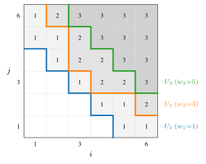
F.2.1 Surrogate Dominance and Nested Tightness
This subsection first proves the nested tightness inequality (Lemma 36), then applies it to prove Lemma 37.
Lemma 36 (Nested Tightness Inequality).
For any $K\geq 1$ and any $z=(z_{1},\ldots,z_{K})\in\{0,1\}^{K}\text{,}$ let $k:=\sum_{r=1}^{K}z_{r}\text{.}$ Then
| $$\sum_{r=1}^{K}(2r-1)\,z_{r}\;\geq\;k^{2},$$ | (75) |
with equality if and only if $z$ is the prefix of length $k\text{,}$ i.e., $z_{1}=\cdots=z_{k}=1$ and $z_{k+1}=\cdots=z_{K}=0\text{.}$
Proof.
At the prefix configuration, equality holds: if $z_{r}=1$ for $r\leq k$ and $z_{r}=0$ for $r>k\text{,}$ then $\sum_{r}(2r-1)\,z_{r}=\sum_{r=1}^{k}(2r-1)=k^{2}$ (the sum of the first $k$ odd numbers).
For general $z\text{,}$ define $S_{1}:=\{r\leq k:z_{r}=0\}$ and $S_{2}:=\{r>k:z_{r}=1\}$ (the “deficit” and “surplus” positions of $z$ relative to the prefix). From
| $$k\;=\;\sum_{r=1}^{K}z_{r}\;=\;\underbrace{(k-|S_{1}|)}_{\sum_{r\leq k}z_{r}}\;+\;\underbrace{|S_{2}|}_{\sum_{r>k}z_{r}},$$ |
we have $|S_{1}|=|S_{2}|\text{.}$ Splitting $\sum_{r}(2r-1)\,z_{r}$ at $r=k\text{,}$
| $$\sum_{r=1}^{K}(2r-1)\,z_{r}\;=\;\!\!\!\sum_{\begin{subarray}{c}r\leq k\\ z_{r}=1\end{subarray}}\!\!\!(2r-1)\,+\,\!\!\!\sum_{\begin{subarray}{c}r>k\\ z_{r}=1\end{subarray}}\!\!\!(2r-1)\;=\;\!\Biggl[\sum_{r=1}^{k}(2r-1)-\sum_{r\in S_{1}}(2r-1)\Biggr]\,+\,\sum_{r\in S_{2}}(2r-1),$$ |
hence
| $$\sum_{r=1}^{K}(2r-1)\,z_{r}\,-\,k^{2}\;=\;\sum_{r\in S_{2}}(2r-1)\,-\,\sum_{r\in S_{1}}(2r-1).$$ | (76) |
Let $|S_{1}|=|S_{2}|=q\text{.}$ For any bijection $\sigma:S_{1}\to S_{2}\text{,}$ the right side of (76) becomes
| $$\sum_{r\in S_{1}}\bigl[(2\sigma(r)-1)-(2r-1)\bigr]\;=\;2\sum_{r\in S_{1}}(\sigma(r)-r).$$ |
For each $r\in S_{1}\text{,}$ $r\leq k<\sigma(r)\text{,}$ so $\sigma(r)-r\geq 1\text{,}$ and summing,
| $$\sum_{r=1}^{K}(2r-1)\,z_{r}\,-\,k^{2}\;=\;2\sum_{r\in S_{1}}(\sigma(r)-r)\;\geq\;2q\;\geq\;0,$$ |
with equality if and only if $q=0\text{,}$ i.e., $S_{1}=S_{2}=\emptyset\text{,}$ i.e., $z$ is the prefix of length $k\text{.}$ ∎
Lemma 37 (Surrogate Dominance and Nested Tightness).
For any $G=(U_{1},\ldots,U_{K})\in\mathcal{U}^{K}$ and any $(x,y)\in[m]^{2}\times[0,1]\text{:}$ (a) Dominance: $\widetilde{\ell}(G;\,x,y)\geq(g_{G}(x)-y)^{2}\text{;}$ (b) Nested tightness: equality if $U_{1}\supseteq U_{2}\supseteq\cdots\supseteq U_{K}\text{.}$
Proof.
Set $z_{r}:=\mathbf{1}\!\left[x\in U_{r}\right]\in\{0,1\}$ and $k:=\sum_{r=1}^{K}z_{r}\text{,}$ so $g_{G}(x)=\tfrac{1}{K}\sum_{r}z_{r}=k/K\text{.}$
Step 1 (Algebraic expansion). From $g_{G}(x)=k/K$ and $\sum_{r=1}^{K}z_{r}=k\text{,}$
| $$(g_{G}(x)-y)^{2}\;=\;\frac{k^{2}}{K^{2}}\,-\,\frac{2ky}{K}\,+\,y^{2}\;=\;\frac{k^{2}}{K^{2}}\,-\,\frac{2y}{K}\sum_{r=1}^{K}z_{r}\,+\,y^{2}.$$ |
On the other hand,
| $$\widetilde{\ell}(G;\,x,y)\;=\;y^{2}\,+\,\sum_{r=1}^{K}\!\left(\frac{2r-1}{K^{2}}-\frac{2y}{K}\right)z_{r}\;=\;y^{2}\,+\,\frac{1}{K^{2}}\sum_{r=1}^{K}(2r-1)\,z_{r}\,-\,\frac{2y}{K}\sum_{r=1}^{K}z_{r}.$$ |
Subtracting, the $y^{2}$ and $\tfrac{2y}{K}\sum_{r}z_{r}$ terms cancel:
| $$\widetilde{\ell}(G;\,x,y)\,-\,(g_{G}(x)-y)^{2}\;=\;\frac{1}{K^{2}}\!\left[\sum_{r=1}^{K}(2r-1)\,z_{r}\,-\,k^{2}\right].$$ | (77) |
Step 2 (Dominance). By Lemma 36, the bracket in (77) is non-negative, so $\widetilde{\ell}(G;\,x,y)\geq(g_{G}(x)-y)^{2}\text{,}$ giving (a).
Step 3 (Nested tightness). If $U_{1}\supseteq U_{2}\supseteq\cdots\supseteq U_{K}\text{,}$ then $z_{r}=\mathbf{1}\!\left[x\in U_{r}\right]$ is non-increasing in $r\text{.}$ Together with $z_{r}\in\{0,1\}\text{,}$ there exists $k^{*}\in\{0,1,\ldots,K\}$ such that $z_{r}=1$ for $r\leq k^{*}$ and $z_{r}=0$ for $r>k^{*}\text{;}$ since $\sum_{r}z_{r}=k\text{,}$ we have $k^{*}=k\text{,}$ so $z$ is the prefix of length $k\text{.}$ By the equality case of Lemma 36, $\sum_{r}(2r-1)\,z_{r}=k^{2}\text{,}$ and (77) gives $\widetilde{\ell}(G;\,x,y)=(g_{G}(x)-y)^{2}\text{,}$ which is (b). ∎
F.2.2 Upset Marginal DP
Lemma 38 (Upset Marginal DP).
Given positive weights $\{w_{ij}\}_{(i,j)\in[m]^{2}}$ and a query $(i_{0},j_{0})\text{,}$ the marginal $p:=\Pr_{U\sim\mu}[(i_{0},j_{0})\in U]$ with $\mu(U)\propto\prod_{(i,j)\in U}w_{ij}\text{,}$ $U\in\mathcal{U}\text{,}$ is computable in $O(m^{2})$ time.
Proof.
Step 1 (Cutoff parametrization). For each row $i\in[m]\text{,}$ define
| $$c_{i}\;:=\;\bigl|\{j\in[m]:(i,j)\notin U\}\bigr|\;\in\;\{0,1,\ldots,m\}.$$ |
Since $U$ is an upset, the set $\{j\in[m]:(i,j)\notin U\}$ is a down-set in $[m]\text{,}$ namely $\{1,2,\ldots,c_{i}\}\text{,}$ so $U\cap(\{i\}\times[m])=\{i\}\times\{c_{i}+1,c_{i}+2,\ldots,m\}\text{,}$ hence
| $$U\;=\;\bigl\{(i,j)\in[m]^{2}:j>c_{i}\bigr\}.$$ | (78) |
The two-dimensional upset constraint ($(i,j)\in U$ and $(i^{\prime},j^{\prime})\succeq(i,j)$ imply $(i^{\prime},j^{\prime})\in U$), specialized to $i^{\prime}=i+1$ and $j^{\prime}=j\text{,}$ requires that $j>c_{i}\Rightarrow j>c_{i+1}$ for all $j\text{,}$ equivalently $c_{i+1}\leq c_{i}\text{.}$ Hence
| $$\mathcal{U}\;\longleftrightarrow\;\bigl\{(c_{1},\ldots,c_{m})\in\{0,1,\ldots,m\}^{m}:c_{1}\geq c_{2}\geq\cdots\geq c_{m}\bigr\}.$$ |
The right side is the set of non-increasing sequences of length $m$ on $\{0,1,\ldots,m\}\text{;}$ by stars-and-bars, the total count is $\binom{2m}{m}\text{,}$ confirming $|\mathcal{U}|=\binom{2m}{m}\text{.}$
Step 2 (Weight factorization and column-tail precomputation). For each row $i\text{,}$ define the column-tail product
| $$a_{i}(c)\;:=\;\prod_{j=c+1}^{m}w_{ij},\qquad c\in\{0,1,\ldots,m\},$$ | (79) |
with the empty product $a_{i}(m)=1\text{.}$ By (78),
| $$\prod_{(i,j)\in U}w_{ij}\;=\;\prod_{i=1}^{m}\prod_{j>c_{i}}w_{ij}\;=\;\prod_{i=1}^{m}a_{i}(c_{i}),$$ |
so $\mu$ factorizes on the cutoff sequence space as
| $$\mu(c_{1},\ldots,c_{m})\;\propto\;\prod_{i=1}^{m}a_{i}(c_{i}),\qquad c_{1}\geq c_{2}\geq\cdots\geq c_{m}.$$ | (80) |
The recursion $a_{i}(m)=1\text{,}$ $a_{i}(c)=a_{i}(c+1)\cdot w_{i,c+1}$ for $c=m-1,m-2,\ldots,0$ takes $O(m)$ per row and $O(m^{2})$ for the full table $\{a_{i}(c)\}_{i,c}\text{.}$
Step 3 (Forward DP). Define
| $$F_{i}(c)\;:=\;\sum_{\begin{subarray}{c}c_{1}\geq\cdots\geq c_{i}=c\\ c_{i^{\prime}}\in\{0,\ldots,m\}\end{subarray}}\prod_{i^{\prime}=1}^{i}a_{i^{\prime}}(c_{i^{\prime}}),\qquad i\in[m],\,c\in\{0,\ldots,m\},$$ | (81) |
i.e., the sum of weights over all non-increasing prefixes $(c_{1},\ldots,c_{i})$ with $c_{i}=c$ (involving all $i$ factors $a_{1},\ldots,a_{i}$).
Base. For $i=1\text{,}$ the sum in (81) reduces to the single point $c_{1}=c\text{,}$ giving $F_{1}(c)=a_{1}(c)\text{.}$
Recursion. For $i\geq 2\text{,}$ grouping by the value $c^{\prime}$ of $c_{i-1}$ (with $c^{\prime}\geq c$),
| $$F_{i}(c)\;=\;a_{i}(c)\cdot\sum_{\begin{subarray}{c}c_{1}\geq\cdots\geq c_{i-1}\geq c\\ c_{i^{\prime}}\in\{0,\ldots,m\}\end{subarray}}\prod_{i^{\prime}=1}^{i-1}a_{i^{\prime}}(c_{i^{\prime}})\;=\;a_{i}(c)\sum_{c^{\prime}\geq c}F_{i-1}(c^{\prime}).$$ | (82) |
The inner sum $\sum_{c^{\prime}\geq c}F_{i-1}(c^{\prime})$ is the suffix sum of $\{F_{i-1}(c^{\prime})\}_{c^{\prime}}\text{;}$ scanning $c$ in descending order while maintaining a running accumulator gives $O(m)$ per row, and multiplying by $a_{i}(c)$ yields $F_{i}(c)$ in $O(m)$ as well, so $F$ takes $O(m^{2})$ in total.
Step 4 (Backward DP). Define
| $$B_{i}(c)\;:=\;\sum_{\begin{subarray}{c}c\geq c_{i+1}\geq c_{i+2}\geq\cdots\geq c_{m}\\ c_{i^{\prime}}\in\{0,\ldots,m\}\end{subarray}}\prod_{i^{\prime}=i+1}^{m}a_{i^{\prime}}(c_{i^{\prime}}),\qquad i\in\{0,1,\ldots,m\},\,c\in\{0,\ldots,m\},$$ | (83) |
i.e., the sum of weights over all non-increasing suffixes $(c_{i+1},\ldots,c_{m})$ with $c_{i+1}\leq c$ (involving the $m{-}i$ factors $a_{i+1},\ldots,a_{m}\text{,}$ but not $a_{i}$).
Base. For $i=m\text{,}$ the sum in (83) reduces to the empty product, giving $B_{m}(c)=1$ for all $c\text{.}$
Recursion. For $i\leq m-1\text{,}$ grouping by the value $c^{\prime}$ of $c_{i+1}$ (with $c^{\prime}\leq c$),
| $$B_{i}(c)\;=\;\sum_{\begin{subarray}{c}c^{\prime}\leq c\\ c^{\prime}\geq c_{i+2}\geq\cdots\geq c_{m}\end{subarray}}a_{i+1}(c^{\prime})\prod_{i^{\prime}=i+2}^{m}a_{i^{\prime}}(c_{i^{\prime}})\;=\;\sum_{c^{\prime}\leq c}a_{i+1}(c^{\prime})\cdot B_{i+1}(c^{\prime}).$$ | (84) |
The inner sum $\sum_{c^{\prime}\leq c}a_{i+1}(c^{\prime})\,B_{i+1}(c^{\prime})$ is the prefix sum of $\{a_{i+1}(c^{\prime})\,B_{i+1}(c^{\prime})\}_{c^{\prime}}\text{;}$ scanning $c$ in ascending order with a running accumulator gives $O(m)$ per row, so $B$ takes $O(m^{2})$ in total.
Step 5 (Marginal formula). For any $i_{0}\in[m]$ and $c\in\{0,\ldots,m\}\text{,}$ fix $c_{i_{0}}=c\text{:}$ the first $i_{0}$ cutoffs satisfy $c_{1}\geq\cdots\geq c_{i_{0}}=c$ with weight sum $F_{i_{0}}(c)$ (involving all $i_{0}$ factors $a_{1},\ldots,a_{i_{0}}$); the last $m-i_{0}$ cutoffs satisfy $c_{i_{0}+1}\leq c$ and $c_{i_{0}+1}\geq\cdots\geq c_{m}$ with weight sum $B_{i_{0}}(c)$ (involving the $m-i_{0}$ factors $a_{i_{0}+1},\ldots,a_{m}\text{,}$ but not $a_{i_{0}}$).
The two segments together cover each of $a_{1},\ldots,a_{m}$ exactly once, so
| $$F_{i_{0}}(c)\cdot B_{i_{0}}(c)\;=\;\sum_{\begin{subarray}{c}c_{1}\geq\cdots\geq c_{m}\\ c_{i_{0}}=c\end{subarray}}\prod_{i=1}^{m}a_{i}(c_{i}).$$ |
Summing over $c$ gives (independent of $i_{0}$)
| $$\sum_{c}F_{i_{0}}(c)\cdot B_{i_{0}}(c)\;=\;\!\!\sum_{c_{1}\geq\cdots\geq c_{m}}\!\!\prod_{i=1}^{m}a_{i}(c_{i})\;=\;Z,$$ | (85) |
where $Z:=\sum_{c_{1}\geq\cdots\geq c_{m}}\prod_{i}a_{i}(c_{i})$ is the partition function of $\mu\text{.}$ In particular, since $B_{m}\equiv 1\text{,}$ $Z=\sum_{c}F_{m}(c)\text{.}$
| $$\Pr_{\mu}\!\bigl[c_{i_{0}}=c\bigr]\;=\;\frac{F_{i_{0}}(c)\cdot B_{i_{0}}(c)}{Z};$$ |
by (78), $(i_{0},j_{0})\in U\Leftrightarrow j_{0}>c_{i_{0}}\Leftrightarrow c_{i_{0}}<j_{0}\text{,}$ so
| $$p\;=\;\Pr_{\mu}\!\bigl[c_{i_{0}}<j_{0}\bigr]\;=\;\frac{1}{Z}\sum_{c<j_{0}}F_{i_{0}}(c)\cdot B_{i_{0}}(c).$$ | (86) |
The sums in the numerator and in $Z=\sum_{c}F_{m}(c)$ are each $O(m)\text{;}$ together with the $O(m^{2})$ precomputation in Steps 2–4, the total time is $O(m^{2})\text{.}$ ∎
F.2.3 Algorithm 2 and Per-Cell EW Equivalence
This subsection formalizes Algorithm 2 and shows that, for each layer $r\in[K]\text{,}$ the per-cell weight update coincides with standard EW on $\mathcal{U}$ with surrogate-coefficient losses $c_{r,t}\text{,}$ learning rate $\eta=1/2\text{,}$ and uniform initialization.
Algorithm 2 (formal restatement).
For each layer $r\in[K]$ and cell $u\in[m]^{2}\text{,}$ maintain a per-cell weight $w_{u,r}^{(t)}>0\text{,}$ initialized as $w_{u,r}^{(1)}:=1\text{.}$ The induced layer-$r$ distribution is
| $$\mu_{t,r}(U)\;\propto\;\prod_{u\in U}w_{u,r}^{(t)},\qquad U\in\mathcal{U},$$ | (87) |
and the global distribution is $\pi_{t}:=\bigotimes_{r=1}^{K}\mu_{t,r}$ on $\mathcal{U}^{K}\text{.}$
At round $t\text{,}$ upon receiving $x_{t}\in[m]^{2}\text{,}$ invoke Lemma 38 on each layer $r$ (with weights $w_{ij}:=w_{(i,j),r}^{(t)}$ and query cell $x_{t}$) to compute
| $$p_{t,r}\;:=\;\Pr_{U\sim\mu_{t,r}}\!\bigl[x_{t}\in U\bigr],\qquad r\in[K];$$ |
predict $\hat{y}_{t}:=\tfrac{1}{K}\sum_{r=1}^{K}p_{t,r}\text{.}$ Upon receiving $y_{t}\in[0,1]\text{,}$ with $c_{r,t}:=(2r-1)/K^{2}-2y_{t}/K\text{,}$ update only the weight at cell $x_{t}\text{:}$
| $$w_{x_{t},r}^{(t+1)}\;:=\;w_{x_{t},r}^{(t)}\cdot\exp\!\left(-\frac{c_{r,t}}{2}\right),\qquad r\in[K],$$ | (88) |
leaving every other cell $u\neq x_{t}$ unchanged, i.e., $w_{u,r}^{(t+1)}:=w_{u,r}^{(t)}\text{.}$
Positivity and time.
Since $w_{u,r}^{(1)}=1>0$ and the update factor $\exp(-c_{r,t}/2)>0\text{,}$ induction gives $w_{u,r}^{(t)}>0$ for all $t\geq 1$ and $(u,r)\text{,}$ so (87) is well-defined and the positivity hypothesis of Lemma 38 is preserved. Each round consists of $K$ invocations of Lemma 38 ($O(Km^{2})$) and prediction and weight updates ($O(K)$), giving $O(Km^{2})$ total per round.
Lemma 39 (Per-Cell EW Equivalence).
For each layer $r\in[K]\text{,}$ the distribution $\mu_{t,r}$ defined by (87) and (88) satisfies $\mu_{1,r}=\mathrm{Unif}(\mathcal{U})\text{,}$ and for all $t\geq 1\text{,}$
| $$\mu_{t+1,r}(U)\;\propto\;\mu_{t,r}(U)\cdot\exp\!\left(-\frac{c_{r,t}}{2}\,\mathbf{1}\!\left[x_{t}\in U\right]\right),\qquad U\in\mathcal{U}.$$ | (89) |
That is, $\mu_{t,r}$ is the Exponential Weights distribution on $\mathcal{U}$ with loss sequence $\{c_{r,s}\,\mathbf{1}\!\left[x_{s}\in\cdot\right]\}_{s<t}\text{,}$ learning rate $\eta=1/2\text{,}$ and uniform initialization.
Proof.
Initial distribution. Since $w_{u,r}^{(1)}=1$ for all $u\text{,}$ $\mu_{1,r}(U)\propto\prod_{u\in U}1=1\text{,}$ and since $|\mathcal{U}|$ is finite, the normalization gives $\mu_{1,r}=\mathrm{Unif}(\mathcal{U})\text{.}$
Per-round equivalence. By (88): $w_{u,r}^{(t+1)}=w_{u,r}^{(t)}\cdot\exp(-c_{r,t}/2)$ for $u=x_{t}\text{,}$ and $w_{u,r}^{(t+1)}=w_{u,r}^{(t)}$ for $u\neq x_{t}\text{.}$ Equivalently, $w_{u,r}^{(t+1)}=w_{u,r}^{(t)}\cdot\xi_{u,t}\text{,}$ where
| $$\xi_{u,t}\;:=\;\begin{cases}\exp(-c_{r,t}/2),&u=x_{t},\\ 1,&u\neq x_{t}.\end{cases}$$ |
Taking the product over $U\in\mathcal{U}\text{,}$
| $$\prod_{u\in U}w_{u,r}^{(t+1)}\;=\;\prod_{u\in U}w_{u,r}^{(t)}\cdot\prod_{u\in U}\xi_{u,t}\;=\;\prod_{u\in U}w_{u,r}^{(t)}\cdot\exp\!\left(-\frac{c_{r,t}}{2}\,\mathbf{1}\!\left[x_{t}\in U\right]\right),$$ |
where the last equality uses $\prod_{u\in U}\xi_{u,t}=\xi_{x_{t},t}^{\mathbf{1}\!\left[x_{t}\in U\right]}=\exp(-c_{r,t}\,\mathbf{1}\!\left[x_{t}\in U\right]/2)$ (only $u=x_{t}$ contributes a non-trivial factor, and only when $x_{t}\in U$). Substituting into (87) gives (89). ∎
Closed form.
Iterating (89) and combining $\sum_{s<t}$ gives the closed form
| $$\mu_{t,r}(U)\;\propto\;\exp\!\left(-\frac{1}{2}\sum_{s<t}c_{r,s}\,\mathbf{1}\!\left[x_{s}\in U\right]\right),\qquad U\in\mathcal{U}.$$ | (90) |
F.2.4 Proof of Theorem 5
Theorem 5 (Surrogate Upper Bound).
Fix any integers $m\geq 2$ and $K\in\mathbb{N}_{+}\text{.}$ Algorithm 2 runs in per-round time $O(Km^{2})$ and, for any sequence $(x_{t},y_{t})_{t=1}^{T}\in[m]^{2}\times[0,1]\text{,}$ satisfies $R_{T}\leq 2K\,\log\!\binom{2m}{m}+T/(4K^{2})\text{.}$ At a level attaining the infimum below, and with $R_{T}\leq T\text{,}$
| $$R_{T}\;\leq\;\min\!\bigl\{T,\;\Psi_{\mathrm{surr}}(T)\bigr\},\quad\Psi_{\mathrm{surr}}(T)\;:=\;\inf_{K\in\mathbb{N}_{+}}\!\biggl\{2K\,\log\!\binom{2m}{m}\,+\,\frac{T}{4K^{2}}\biggr\}.$$ | (6) |
Proof.
Attainment. The objective defining $\Psi_{\mathrm{surr}}$ tends to infinity with $K\text{,}$ and its infimum is attained.
Per-round time. Established in Section F.2.3 as $O(Km^{2})\text{.}$
Regret bound. Since $\pi_{t}=\bigotimes_{r}\mu_{t,r}$ and $g_{G}(x_{t})=\tfrac{1}{K}\sum_{r}\mathbf{1}\!\left[x_{t}\in U_{r}\right]\text{,}$
| $$\hat{y}_{t}\;=\;\tfrac{1}{K}\sum_{r=1}^{K}p_{t,r}\;=\;\tfrac{1}{K}\sum_{r=1}^{K}\mathbb{E}_{U\sim\mu_{t,r}}\!\bigl[\mathbf{1}\!\left[x_{t}\in U\right]\bigr]\;=\;\mathbb{E}_{G\sim\pi_{t}}\!\bigl[g_{G}(x_{t})\bigr].$$ |
Step 1 (Exp-concavity and Jensen). The map $p\mapsto\exp(-\tfrac{1}{2}(p-y_{t})^{2})$ is concave on $p\in[0,1]$ (the squared loss is $\tfrac{1}{2}$-exp-concave); by Jensen’s inequality,
| $$\exp\!\left(-\tfrac{1}{2}(\hat{y}_{t}-y_{t})^{2}\right)\;=\;\exp\!\left(-\tfrac{1}{2}\!\left(\mathbb{E}_{G\sim\pi_{t}}[g_{G}(x_{t})]-y_{t}\right)^{2}\right)\;\geq\;\mathbb{E}_{G\sim\pi_{t}}\!\left[\exp\!\left(-\tfrac{1}{2}(g_{G}(x_{t})-y_{t})^{2}\right)\right].$$ |
Taking $-2\log$ of both sides (which reverses the inequality):
| $$(\hat{y}_{t}-y_{t})^{2}\;\leq\;-2\log\,\mathbb{E}_{G\sim\pi_{t}}\!\left[\exp\!\left(-\tfrac{1}{2}(g_{G}(x_{t})-y_{t})^{2}\right)\right].$$ | (91) |
Step 2 (Surrogate replacement). By Lemma 37(a), $\widetilde{\ell}_{t}(G)\geq(g_{G}(x_{t})-y_{t})^{2}\text{,}$ so $\exp(-\widetilde{\ell}_{t}(G)/2)\leq\exp(-(g_{G}(x_{t})-y_{t})^{2}/2)\text{;}$ taking the $\pi_{t}$-expectation preserves the inequality, and applying $-2\log$ reverses it:
| $$(\hat{y}_{t}-y_{t})^{2}\;\leq\;-2\log\,\mathbb{E}_{G\sim\pi_{t}}\!\left[\exp\!\left(-\tfrac{1}{2}\widetilde{\ell}_{t}(G)\right)\right].$$ | (92) |
Step 3 (Layer-wise telescoping). By the layer-wise additivity $\widetilde{\ell}_{s}(G)=y_{s}^{2}+\sum_{r}c_{r,s}\,\mathbf{1}\!\left[x_{s}\in U_{r}\right]$ and Lemma 39 (specifically (90)),
| $$\begin{split}\pi_{t}(G)&\;=\;\prod_{r=1}^{K}\mu_{t,r}(U_{r})\;\propto_{G}\;\prod_{r=1}^{K}\exp\!\left(-\tfrac{1}{2}\sum_{s<t}c_{r,s}\,\mathbf{1}\!\left[x_{s}\in U_{r}\right]\right)\\ &\;=\;\exp\!\left(-\tfrac{1}{2}\sum_{s<t}\sum_{r=1}^{K}c_{r,s}\,\mathbf{1}\!\left[x_{s}\in U_{r}\right]\right).\end{split}$$ | (93) |
Define the cumulative weight and partition function (with base distribution $\pi_{1}=\bigotimes_{r}\mathrm{Unif}(\mathcal{U})=\mathrm{Unif}(\mathcal{U}^{K})$):
| $$W_{t}(G)\;:=\;\exp\!\left(-\tfrac{1}{2}\sum_{s<t}\widetilde{\ell}_{s}(G)\right),\qquad Z_{t}\;:=\;\mathbb{E}_{G\sim\pi_{1}}\!\bigl[W_{t}(G)\bigr],$$ |
with the empty-sum convention, so $W_{1}\equiv 1$ and $Z_{1}=1\text{.}$ Since $\sum_{s<t}y_{s}^{2}$ is independent of $G\text{,}$
| $$W_{t}(G)\;=\;\exp\!\left(-\tfrac{1}{2}\sum_{s<t}y_{s}^{2}\right)\cdot\exp\!\left(-\tfrac{1}{2}\sum_{s<t}\sum_{r}c_{r,s}\,\mathbf{1}\!\left[x_{s}\in U_{r}\right]\right)\;\propto_{G}\;\pi_{t}(G),$$ |
where the last step uses (93). After normalization, $\pi_{t}(G)=\pi_{1}(G)\,W_{t}(G)/Z_{t}\text{.}$
By the standard EW potential argument,
| $$\mathbb{E}_{G\sim\pi_{t}}\!\left[\exp\!\left(-\tfrac{1}{2}\widetilde{\ell}_{t}(G)\right)\right]\;=\;\frac{1}{Z_{t}}\mathbb{E}_{G\sim\pi_{1}}\!\left[W_{t}(G)\exp\!\left(-\tfrac{1}{2}\widetilde{\ell}_{t}(G)\right)\right]\;=\;\frac{\mathbb{E}_{\pi_{1}}[W_{t+1}(G)]}{Z_{t}}\;=\;\frac{Z_{t+1}}{Z_{t}}.$$ |
Substituting into (92) and summing over $t=1,\ldots,T$ (telescoping),
| $$\sum_{t=1}^{T}(\hat{y}_{t}-y_{t})^{2}\;\leq\;-2\sum_{t=1}^{T}\log\frac{Z_{t+1}}{Z_{t}}\;=\;-2\log\frac{Z_{T+1}}{Z_{1}}\;=\;-2\log Z_{T+1},$$ |
where the last equality uses $Z_{1}=1\text{.}$
To lower-bound $Z_{T+1}\text{:}$ for any $G^{*}\in\mathcal{U}^{K}\text{,}$ since $\pi_{1}(G^{*})=\binom{2m}{m}^{-K}\text{,}$
| $$Z_{T+1}\;=\;\mathbb{E}_{G\sim\pi_{1}}[W_{T+1}(G)]\;\geq\;\pi_{1}(G^{*})\cdot W_{T+1}(G^{*})\;=\;\binom{2m}{m}^{-K}\exp\!\left(-\tfrac{1}{2}\sum_{t=1}^{T}\widetilde{\ell}_{t}(G^{*})\right).$$ |
Applying $-2\log$ (which reverses the direction):
| $$\sum_{t=1}^{T}(\hat{y}_{t}-y_{t})^{2}\;\leq\;-2\log Z_{T+1}\;\leq\;\sum_{t=1}^{T}\widetilde{\ell}_{t}(G^{*})\,+\,2K\log\!\binom{2m}{m}.$$ | (94) |
Step 4 (Comparator selection and Block Residual). Take
| $$f^{*}\;\in\;\operatorname*{arg\,min}_{f\in\mathcal{F}_{[m]^{2}}^{\uparrow}}\sum_{t=1}^{T}\bigl(f(x_{t})-y_{t}\bigr)^{2},$$ |
and let $q:[0,1]\to\{0,1/K,\ldots,1\}\text{,}$ $q(v):=\lfloor Kv+1/2\rfloor/K\text{,}$ denote rounding to the $K$-grid; set $\hat{f}:=q\circ f^{*}\text{.}$ Since $q$ is non-decreasing and $f^{*}$ is isotonic, $\hat{f}$ is isotonic and takes values in $\{0,1/K,\ldots,1\}\text{.}$
Define the nested upset sequence
| $$U_{r}^{*}\;:=\;\bigl\{u\in[m]^{2}:\hat{f}(u)\geq r/K\bigr\},\qquad r\in[K].$$ |
Since $\hat{f}$ is isotonic, each $U_{r}^{*}$ is an upset of $[m]^{2}\text{;}$ since $r/K$ is strictly increasing in $r\text{,}$ $U_{1}^{*}\supseteq U_{2}^{*}\supseteq\cdots\supseteq U_{K}^{*}\text{.}$ Set $G^{*}:=(U_{1}^{*},\ldots,U_{K}^{*})\in\mathcal{U}^{K}\text{.}$
Identifying $g_{G^{*}}$ with $\hat{f}\text{.}$ For any $u\in[m]^{2}\text{,}$ since $\hat{f}(u)\in\{0,1/K,\ldots,1\}\text{,}$ there is a unique $k\in\{0,1,\ldots,K\}$ with $\hat{f}(u)=k/K\text{.}$ Then
| $$\mathbf{1}\!\left[u\in U_{r}^{*}\right]\;=\;\mathbf{1}\!\left[\hat{f}(u)\geq r/K\right]\;=\;\mathbf{1}\!\left[k\geq r\right],$$ |
so
| $$g_{G^{*}}(u)\;=\;\tfrac{1}{K}\sum_{r=1}^{K}\mathbf{1}\!\left[u\in U_{r}^{*}\right]\;=\;\tfrac{1}{K}\cdot\bigl|\{r\in[K]:r\leq k\}\bigr|\;=\;\tfrac{k}{K}\;=\;\hat{f}(u).$$ |
Applying Lemma 37(b). Since $G^{*}$ is nested, Lemma 37(b) gives $\widetilde{\ell}_{t}(G^{*})=(g_{G^{*}}(x_{t})-y_{t})^{2}=(\hat{f}(x_{t})-y_{t})^{2}\text{;}$ substituting into (94),
| $$\sum_{t=1}^{T}(\hat{y}_{t}-y_{t})^{2}\;\leq\;\sum_{t=1}^{T}\bigl(\hat{f}(x_{t})-y_{t}\bigr)^{2}\,+\,2K\log\!\binom{2m}{m}.$$ | (95) |
Discretization error. For each value $c$ attained by $f^{*}\text{,}$ let $\delta_{c}:=q(c)-c\text{;}$ since $q$ rounds to the nearest grid point, $|\delta_{c}|\leq 1/(2K)\text{,}$ so $\hat{f}(u)=q(f^{*}(u))=f^{*}(u)+\delta_{f^{*}(u)}\text{.}$ Define the query counts and blocks
| $$w_{u}\;:=\;\bigl|\{t\in[T]:x_{t}=u\}\bigr|,\qquad B_{c}\;:=\;\bigl\{u\in[m]^{2}:w_{u}>0,\,f^{*}(u)=c\bigr\}.$$ |
Applying Lemma 8 (Block Residual) on the poset $\mathcal{P}=[m]^{2}$ with sequence $(x_{t},y_{t})_{t=1}^{T}$ and minimizer $f^{*}\text{:}$ for each value $c\text{,}$
| $$\!\!\sum_{t\,:\,x_{t}\in B_{c}}\!\!\bigl(f^{*}(x_{t})-y_{t}\bigr)\;=\;0.$$ | (96) |
Decomposing the loss difference between $\hat{f}$ and $f^{*}$ by block: for $u\in B_{c}\text{,}$ $f^{*}(u)=c$ and $\hat{f}(u)=c+\delta_{c}\text{,}$ so for $t:x_{t}\in B_{c}\text{,}$
| $$\bigl(\hat{f}(x_{t})-y_{t}\bigr)^{2}-\bigl(f^{*}(x_{t})-y_{t}\bigr)^{2}\;=\;(c+\delta_{c}-y_{t})^{2}-(c-y_{t})^{2}\;=\;\delta_{c}^{2}+2\,\delta_{c}\,(c-y_{t}).$$ |
Summing over $\{t:x_{t}\in B_{c}\}$ (with $w_{B_{c}}:=\sum_{u\in B_{c}}w_{u}$),
| $$\!\!\sum_{t\,:\,x_{t}\in B_{c}}\!\!\bigl[(\hat{f}(x_{t})-y_{t})^{2}-(f^{*}(x_{t})-y_{t})^{2}\bigr]\;=\;w_{B_{c}}\,\delta_{c}^{2}\,+\,2\,\delta_{c}\underbrace{\sum_{t\,:\,x_{t}\in B_{c}}(c-y_{t})}_{=\,0\text{ by }\text{(96)}},$$ |
where $c=f^{*}(x_{t})$ for $x_{t}\in B_{c}\text{.}$ Summing over $c$ (with $\sum_{c}w_{B_{c}}=\sum_{u}w_{u}=T$),
| $$\sum_{t=1}^{T}\!\bigl[(\hat{f}(x_{t})-y_{t})^{2}-(f^{*}(x_{t})-y_{t})^{2}\bigr]\;=\;\sum_{c}w_{B_{c}}\,\delta_{c}^{2}\;\leq\;\frac{T}{4K^{2}},$$ | (97) |
where the final inequality uses $\delta_{c}^{2}\leq 1/(4K^{2})\text{.}$
| $$R_{T}\;=\;\sum_{t=1}^{T}(\hat{y}_{t}-y_{t})^{2}\,-\,\sum_{t=1}^{T}\bigl(f^{*}(x_{t})-y_{t}\bigr)^{2}\;\leq\;2K\log\!\binom{2m}{m}\,+\,\frac{T}{4K^{2}}.$$ |
This holds for any $K\in\mathbb{N}_{+}\text{,}$ so $R_{T}\leq\Psi_{\mathrm{surr}}(T)\text{.}$
Trivial bound. Since $\hat{y}_{t},y_{t}\in[0,1]\text{,}$ $(\hat{y}_{t}-y_{t})^{2}\leq 1$ per round; combined with $\min_{f^{*}\in\mathcal{F}_{[m]^{2}}^{\uparrow}}\sum_{t}(f^{*}(x_{t})-y_{t})^{2}\geq 0\text{,}$ $R_{T}\leq T\text{.}$ Taking the minimum yields $R_{T}\leq\min\{T,\Psi_{\mathrm{surr}}(T)\}\text{.}$ ∎
F.3 Combined Upper Bound and Horizon-Free Wrapper
This appendix gives the complete proofs of Theorem 40 (Combined Upper Bound) and Theorem 6 (Horizon-Free Polynomial-Time Rate-Optimal Algorithm). The argument has three steps: (i) Section F.3.1 obtains Theorem 40 as the minimum of Theorem 35, Theorem 5, and the trivial $T$ bound, and establishes that $\Phi(T):=\min\{T,\Psi_{\mathrm{col}}(T),\Psi_{\mathrm{surr}}(T)\}$ satisfies the five properties required by the generic wrapper framework (Lemma 41); (ii) Section F.3.2 abstracts the generic $\Phi$-wrapper framework (Lemma 42), proving that for any $\Phi$ satisfying these five properties and any base algorithm class satisfying the base regret hypothesis, the epoch-restart wrapper gives $R_{T}\leq 4\Phi(T)+2\text{;}$ (iii) Section F.3.3 formalizes Algorithm 3 and applies Lemma 42 to the specific $\Phi$ and base algorithms (Algorithm 1, Algorithm 2) of Section 5.3 to obtain Theorem 6; the per-round time $\mathrm{poly}(m,t)$ is established directly via the polynomial growth of base per-round time in the horizon $L$ and the polynomial $(m,t)$-bound on $L_{k}\text{.}$
Recall.
We use the following notation. $\mathcal{F}_{[m]^{2}}^{\uparrow}$ denotes the class of $[0,1]$-valued isotonic functions on $[m]^{2}\text{;}$ $\Phi(T):=\min\{T,\Psi_{\mathrm{col}}(T),\Psi_{\mathrm{surr}}(T)\}$ is the lower-envelope regret bound, with $\Psi_{\mathrm{col}}(T)=\inf_{K\in\mathbb{N}_{+}}\{2m\log\binom{m+K}{K}+T/(4K^{2})\}$ and $\Psi_{\mathrm{surr}}(T)=\inf_{K\in\mathbb{N}_{+}}\{2K\log\binom{2m}{m}+T/(4K^{2})\}$ given by Theorems 35 and 5 as inf-of-affine forms; $L_{k}:=\max\{L\in\mathbb{N}_{+}:\Phi(L)\leq 2^{k-1}\}$ is the last-below epoch length (8); $T_{j}:=\sum_{k\leq j}L_{k}$ ($T_{0}:=0$) is the cumulative epoch length; and $W^{\Phi}$ denotes the epoch-restart wrapper described in Algorithm 3. Within epoch $k$ (i.e., $T_{k-1}<t\leq T_{k}$), the wrapper selects the base algorithm $A_{k}$ to be Algorithm 1 with $K^{*}=K^{*}_{\mathrm{col}}(L_{k})$ if $\Psi_{\mathrm{col}}(L_{k})\leq\Psi_{\mathrm{surr}}(L_{k})\text{,}$ and Algorithm 2 with $K^{*}=K^{*}_{\mathrm{surr}}(L_{k})$ otherwise; $A_{k}$ is freshly initialized at the start of each epoch and shares no state across epochs.
F.3.1 Combined Upper Bound
This subsection proves Theorem 40 and establishes the five properties of $\Phi$ (Lemma 41).
Theorem 40 (Combined Upper Bound).
For any $m\geq 2\text{,}$ $T\geq 1\text{,}$ and any sequence $(x_{t},y_{t})_{t=1}^{T}\in[m]^{2}\times[0,1]\text{,}$ the combined strategy runs in $\mathrm{poly}(m,T)$ per-round time and satisfies $R_{T}\leq\Phi(T)\text{.}$
Proof.
Theorem 35 (specialized to $K^{*}=K^{*}_{\mathrm{col}}(T)$) gives $R_{T}\leq\Psi_{\mathrm{col}}(T)\text{,}$ and Theorem 5 (specialized to $K^{*}=K^{*}_{\mathrm{surr}}(T)$) gives $R_{T}\leq\Psi_{\mathrm{surr}}(T)\text{.}$ The combined strategy chooses the smaller of the two depending on whether $\Psi_{\mathrm{col}}(T)\leq\Psi_{\mathrm{surr}}(T)$ and runs the chosen algorithm over the entire sequence, so the resulting regret satisfies $R_{T}\leq\min\{\Psi_{\mathrm{col}}(T),\Psi_{\mathrm{surr}}(T)\}\text{.}$ Together with the trivial bound $R_{T}\leq T$ (since $\hat{y}_{t},y_{t}\in[0,1]$ implies a per-round squared loss at most $1$ and the isotonic comparator loss is non-negative), taking the minimum of the three gives $R_{T}\leq\Phi(T)\text{.}$ The per-round time is polynomial in $(m,T)\text{:}$ Algorithm 1 runs in $O(mK^{*}_{\mathrm{col}}(T))$ per round (Lemma 32); Algorithm 2 runs in $O(K^{*}_{\mathrm{surr}}(T)\,m^{2})$ per round (Section F.2.3); and both $K^{*}_{\mathrm{col}}(T)$ and $K^{*}_{\mathrm{surr}}(T)$ are polynomial in $(m,T)$ (concretely, $K^{*}_{\mathrm{col}}(T)\leq O(\sqrt{T}/m+(T/m)^{1/3}+1)$ and $K^{*}_{\mathrm{surr}}(T)\leq O((T/m)^{1/3}+1)\text{;}$ see Sections 5.1 and 5.2). ∎
Lemma 41 (Properties of $\Phi$).
$\Phi(T)=\min\{T,\Psi_{\mathrm{col}}(T),\Psi_{\mathrm{surr}}(T)\}$ satisfies, on $\mathbb{R}_{+}\text{,}$
- (P1)
$\Phi(0)=0$;
- (P2)
$\Phi$ is non-decreasing;
- (P3)
$\Phi$ is concave;
- (P4)
$\Phi$ is unbounded: $\lim_{T\to\infty}\Phi(T)=\infty$;
- (P5)
$\Phi(L+1)-\Phi(L)\leq 1$ for all $L\in\mathbb{N}$ (i.e., $1$-Lipschitz on $\mathbb{N}$).
Proof.
We address each property in turn.
(P1). At $T=0\text{:}$ $\Psi_{\mathrm{col}}(0)=\inf_{K\in\mathbb{N}_{+}}\{2m\log\binom{m+K}{K}\}=2m\log(m+1)>0$ (the minimum is attained at $K=1$); and $\Psi_{\mathrm{surr}}(0)=\inf_{K\in\mathbb{N}_{+}}\{2K\log\binom{2m}{m}\}=2\log\binom{2m}{m}>0$ (also at $K=1$). Hence $\Phi(0)=\min\{0,\Psi_{\mathrm{col}}(0),\Psi_{\mathrm{surr}}(0)\}=0\text{.}$
(P2). Each of the three terms is non-decreasing in $T\text{:}$ $T\mapsto T$ is trivial; $\Psi_{\mathrm{col}}(T)=\inf_{K}[a_{K}+T/(4K^{2})]$ (with $a_{K}:=2m\log\binom{m+K}{K}$), each $K$-th term is affine in $T$ with slope $1/(4K^{2})>0\text{,}$ and the infimum preserves non-decreasingness (for $T_{1}\leq T_{2}\text{,}$ $\inf_{K}f_{K}(T_{1})\leq f_{K}(T_{1})\leq f_{K}(T_{2})$ for each $K\text{,}$ so $\inf_{K}f_{K}(T_{1})\leq\inf_{K}f_{K}(T_{2})$); $\Psi_{\mathrm{surr}}$ is analogous. The minimum of non-decreasing functions is non-decreasing (for $T_{1}\leq T_{2}$ and WLOG $f(T_{1})\leq g(T_{1})\text{,}$ $\min(f,g)(T_{1})=f(T_{1})\leq f(T_{2})$ and $f(T_{1})\leq g(T_{1})\leq g(T_{2})\text{,}$ so $f(T_{1})\leq\min(f,g)(T_{2})$).
(P3). Each of the three terms is concave: $T\mapsto T$ is linear, hence concave; $\Psi_{\mathrm{col}}$ and $\Psi_{\mathrm{surr}}$ are infima of affine families in $T$ (write as $\inf_{K}[a_{K}+b_{K}T]\text{,}$ with the appropriate $a_{K},b_{K}$), and the standard inf-of-affine computation gives concavity: for $\alpha\in[0,1]$ and $T_{1},T_{2}\in\mathbb{R}_{+}\text{,}$
| $$\Psi(\alpha T_{1}+(1-\alpha)T_{2})\;=\;\inf_{K}\bigl[\alpha(a_{K}+b_{K}T_{1})+(1-\alpha)(a_{K}+b_{K}T_{2})\bigr]\;\geq\;\alpha\,\Psi(T_{1})+(1-\alpha)\,\Psi(T_{2}),$$ |
where the inequality uses $\inf_{K}[\alpha A_{K}+(1-\alpha)B_{K}]\geq\alpha\inf_{K}A_{K}+(1-\alpha)\inf_{K}B_{K}\text{.}$ The minimum preserves concavity: if $f,g$ are concave, then by the concavity of $f$ and $\min(f,g)\leq f\text{,}$
| $$f(\alpha T_{1}+(1-\alpha)T_{2})\;\geq\;\alpha\,f(T_{1})+(1-\alpha)\,f(T_{2})\;\geq\;\alpha\,\min(f,g)(T_{1})+(1-\alpha)\,\min(f,g)(T_{2}),$$ |
and analogously for $g\text{.}$ Taking the smaller of the two yields $\min(f,g)(\alpha T_{1}+(1-\alpha)T_{2})\geq\alpha\,\min(f,g)(T_{1})+(1-\alpha)\,\min(f,g)(T_{2})\text{,}$ i.e., $\min(f,g)$ is concave. Combining the three concave terms with the concavity-preserving minimum, $\Phi$ is concave.
(P4). Each of the three terms is unbounded: the identity $T\mapsto T$ is unbounded; by the phase-wise rates of Sections 5.1 and 5.2, $\Psi_{\mathrm{col}}(T)=\Theta\bigl(m^{2}\log(T/m^{4})\bigr)$ in Phase 2, hence $\to\infty\text{;}$ and $\Psi_{\mathrm{surr}}(T)=\Theta(m^{2/3}T^{1/3})$ in Phases 1 and 2, $\to\infty\text{.}$ The minimum of three diverging functions diverges, so $\Phi(T)\to\infty\text{.}$
(P5). By (P3) (concavity), the difference $\Delta_{L}:=\Phi(L+1)-\Phi(L)$ is non-increasing in $L\in\mathbb{N}\text{:}$ for $L_{1}\leq L_{2}\text{,}$ concavity implies that the average slope of $\Phi$ on $[L_{1},L_{1}+1]$ is at least that on $[L_{2},L_{2}+1]\text{,}$ so $\Delta_{L_{1}}\geq\Delta_{L_{2}}\text{.}$ In particular, $\Delta_{L}\leq\Delta_{0}=\Phi(1)-\Phi(0)=\Phi(1)$ (using (P1) $\Phi(0)=0$). Moreover, $\Phi(1)=\min\{1,\Psi_{\mathrm{col}}(1),\Psi_{\mathrm{surr}}(1)\}\leq 1$ (using the $T=1$ term), so $\Delta_{L}\leq 1$ for all $L\in\mathbb{N}\text{.}$ ∎
F.3.2 Generic $\Phi$-Wrapper Framework
This subsection abstracts the wrapper framework into a form independent of the specific $\Phi$ and base algorithms: given a $\Phi$ satisfying (P1)–(P5) and a class of base algorithms $\{A^{L}\}$ satisfying the base regret hypothesis, the wrapper with last-below epoch partitioning and base restart yields a horizon-free regret bound $4\Phi(T)+2\text{.}$ Section F.3.3 applies this framework to the specific $\Phi$ and Algorithm 1, Algorithm 2 of Section 5.3.
Setup.
Suppose $\Phi:\mathbb{R}_{+}\to\mathbb{R}_{+}$ satisfies properties (P1)–(P5) of Lemma 41. Given a base algorithm class $\{A^{L}\}_{L\in\mathbb{N}_{+}}\text{,}$ where $A^{L}$ is an online algorithm taking horizon $L$ as input, satisfying the base regret hypothesis: for any sequence $(x_{s},y_{s})_{s=1}^{L}\in[m]^{2}\times[0,1]$ and any $\tau\in[1,L]\text{,}$
| $$R_{\tau}(A^{L})\;:=\;\sum_{s=1}^{\tau}(\hat{y}_{s}-y_{s})^{2}\,-\,\min_{f\in\mathcal{F}_{[m]^{2}}^{\uparrow}}\sum_{s=1}^{\tau}\bigl(f(x_{s})-y_{s}\bigr)^{2}\;\leq\;\Phi(L),$$ | (98) |
where $\hat{y}_{s}$ is the prediction of $A^{L}$ at round $s\text{.}$ The $\Phi$-wrapper $W^{\Phi}$ proceeds via last-below epoch partitioning and base restart: define epoch $k\in\mathbb{N}_{+}$ length
| $$L_{k}\;:=\;\max\bigl\{L\in\mathbb{N}_{+}:\Phi(L)\leq 2^{k-1}\bigr\},$$ |
and cumulative length $T_{j}:=\sum_{k\leq j}L_{k}$ ($T_{0}:=0$); within epoch $k$ (i.e., $T_{k-1}<t\leq T_{k}$), run a fresh instance of $A^{L_{k}}\text{,}$ with no state shared across epochs.
Lemma 42 (Generic $\Phi$-Wrapper Regret).
Suppose $\Phi$ satisfies (P1)–(P5) and the base algorithm class $\{A^{L}\}$ satisfies (98). Then the wrapper $W^{\Phi}\text{,}$ for any $T\geq 1$ and any sequence $(x_{t},y_{t})_{t=1}^{T}\in[m]^{2}\times[0,1]\text{,}$ satisfies
| $$R_{T}(W^{\Phi})\;\leq\;4\Phi(T)+2.$$ | (99) |
Proof.
The argument has two steps: first, $L_{k}$ is well-defined and $L_{k}\geq 1\text{;}$ then we accumulate the regret across epochs.
Step 1 ($L_{k}$ well-defined; $L_{k}\geq 1$). Let $S_{k}:=\{L\in\mathbb{N}_{+}:\Phi(L)\leq 2^{k-1}\}\text{.}$ By (P5) and (P1), $\Phi(1)-\Phi(0)\leq 1$ and $\Phi(0)=0$ give $\Phi(1)\leq 1\leq 2^{k-1}$ for all $k\geq 1\text{,}$ so $1\in S_{k}$ and $S_{k}$ is non-empty. By (P4), there exists $L^{*}\in\mathbb{N}_{+}$ with $\Phi(L^{*})>2^{k-1}\text{;}$ combined with (P2), $\Phi$ is non-decreasing, so $S_{k}\subseteq\{1,2,\ldots,L^{*}-1\}\text{,}$ and $S_{k}$ is finite. Hence $L_{k}=\max S_{k}$ is well-defined and $L_{k}\geq 1\text{.}$
Step 2 (Regret accumulation). Suppose $T\in(T_{K-1},T_{K}]$ (i.e., $T$ falls within epoch $K$). The wrapper runs a fresh instance $A^{L_{k}}_{k}$ within epoch $k\text{,}$ producing predictions on the sub-sequence $(x_{s},y_{s})$ for $T_{k-1}<s\leq\min(T_{k},T)\text{.}$ By the sub-additivity of the isotonic-class minimum loss across epoch partitioning—i.e., for any partitioning of $1,\ldots,T$ into epochs,
| $$\min_{f\in\mathcal{F}_{[m]^{2}}^{\uparrow}}\sum_{s=1}^{T}\bigl(f(x_{s})-y_{s}\bigr)^{2}\;\geq\;\sum_{k=1}^{K}\min_{f_{k}\in\mathcal{F}_{[m]^{2}}^{\uparrow}}\!\!\sum_{s\in\text{epoch }k}\!\!\bigl(f_{k}(x_{s})-y_{s}\bigr)^{2}$$ |
(per-epoch comparators are more flexible than a single global comparator)—the wrapper’s regret is bounded above by the sum of per-epoch regrets:
| $$R_{T}(W^{\Phi})\;\leq\;\sum_{k=1}^{K-1}R_{L_{k}}\bigl(A^{L_{k}}_{k}\bigr)+R_{T-T_{K-1}}\bigl(A^{L_{K}}_{K}\bigr).$$ |
By (98) (with epoch length $L_{k}$ and final segment length $T-T_{K-1}\leq L_{K}$), each term is at most $\Phi(L_{k})\text{;}$ by $L_{k}\in S_{k}\text{,}$ $\Phi(L_{k})\leq 2^{k-1}\text{.}$ Summing,
| $$R_{T}\;\leq\;\sum_{k=1}^{K}\Phi(L_{k})\;\leq\;\sum_{k=1}^{K}2^{k-1}\;=\;2^{K}-1.$$ | (100) |
We control $2^{K}-1$ in terms of $\Phi(T)\text{.}$
Case 1 ($K=1$). Then $T\in(0,L_{1}]\text{,}$ so by (100) $R_{T}\leq 2^{1}-1=1\text{.}$ By (P1) and (P2), $\Phi(T)\geq\Phi(0)=0\text{,}$ so $4\Phi(T)+2\geq 2>1\geq R_{T}\text{.}$
Case 2 ($K\geq 2$). Then $T\geq T_{K-1}+1\geq L_{K-1}+1$ (using $T_{K-1}=\sum_{k\leq K-1}L_{k}\geq L_{K-1}$). By the maximality of $L_{K-1}\text{,}$ $L_{K-1}+1\notin S_{K-1}\text{,}$ i.e., $\Phi(L_{K-1}+1)>2^{K-2}\text{.}$ Combined with (P2) and $T\geq L_{K-1}+1\text{,}$
| $$\Phi(T)\;\geq\;\Phi(L_{K-1}+1)\;>\;2^{K-2},$$ |
i.e., $4\Phi(T)>2^{K}\text{.}$ Hence by (100) $R_{T}\leq 2^{K}-1<4\Phi(T)-1\leq 4\Phi(T)+2\text{.}$
Combining the two cases, $R_{T}(W^{\Phi})\leq 4\Phi(T)+2\text{.}$ ∎
F.3.3 Proof of Theorem 6
This subsection applies Lemma 42 to the specific $\Phi$ and base algorithms (Algorithm 1, Algorithm 2) of Section 5.3 to obtain Theorem 6. Algorithm 3 is the specialization of $W^{\Phi}$ to $\Phi(T)=\min\{T,\Psi_{\mathrm{col}}(T),\Psi_{\mathrm{surr}}(T)\}$ described in Section 5.3.
Algorithm 3 (formal restatement).
Given edge length $m\text{,}$ the wrapper maintains the current epoch index $k\text{,}$ intra-epoch round $\tau\text{,}$ and global round $t\text{,}$ initialized as $k:=1\text{,}$ $\tau:=0\text{,}$ $t:=0\text{,}$ and $L_{1}:=\max\{L\in\mathbb{N}_{+}:\Phi(L)\leq 1\}=1$ (in Phase 0 where $\Phi(L)=L$ for $L\leq m\text{;}$ well-definedness follows from Lemma 42, Step 1). The wrapper selects $A_{1}$ to be Algorithm 1 with $K^{*}=K^{*}_{\mathrm{col}}(L_{1})$ if $\Psi_{\mathrm{col}}(L_{1})\leq\Psi_{\mathrm{surr}}(L_{1})\text{,}$ and Algorithm 2 with $K^{*}=K^{*}_{\mathrm{surr}}(L_{1})$ otherwise, freshly initialized. Before each round, the wrapper checks for an epoch transition: if $\tau=L_{k}\text{,}$ it sets $k\leftarrow k+1\text{,}$ $\tau\leftarrow 0\text{,}$ $L_{k}\leftarrow\max\{L\in\mathbb{N}_{+}:\Phi(L)\leq 2^{k-1}\}\text{,}$ re-selects $A_{k}$ according to the same rule, and freshly initializes it. Then $\tau\leftarrow\tau+1$ and $t\leftarrow t+1\text{;}$ $A_{k}$ outputs $\hat{y}_{t}$ on its $\tau$-th round upon receiving $x_{t}\text{,}$ then updates its internal state (via the rule (58) for Algorithm 1 or the layer-wise EW update of Section 5.2 for Algorithm 2) upon receiving $y_{t}\in[0,1]\text{.}$ The wrapper does not access any external horizon information; its decision at each round depends only on $(k,\tau,L_{k})$ and the state of $A_{k}\text{.}$
Theorem 6 (Horizon-Free Polynomial-Time Rate-Optimal Algorithm).
Algorithm 3 runs in $\mathrm{poly}(m,t)$ per-round time at every round $t\geq 1$ and, for any $T\geq 1$ and any sequence $(x_{t},y_{t})_{t=1}^{T}\in[m]^{2}\times[0,1]\text{,}$ satisfies $R_{T}\leq 4\,\Phi(T)+2\text{.}$
Proof.
We prove the per-round time and regret bounds separately.
Per-round time. Within epoch $k\text{,}$ the wrapper runs the base algorithm $A_{k}$ (Algorithm 1 or Algorithm 2) with horizon $L_{k}\text{,}$ at per-round time polynomial in $(m,L_{k})$ (Theorem 40). We show $L_{k}$ is polynomially bounded in $(m,t)\text{,}$ so the per-round time is polynomial in $(m,t)\text{.}$
For $k=1\text{,}$ $L_{1}=1$ (as in the formal restatement), so the per-round time is $\mathrm{poly}(m,1)=\mathrm{poly}(m)\text{,}$ which is therefore polynomial in $(m,t)\text{.}$
For $k\geq 2\text{,}$ in epoch $k$ we have $t\geq T_{k-1}+1\geq L_{k-1}+1\text{.}$ By the maximality of $L_{k-1}\text{,}$ $\Phi(L_{k-1}+1)>2^{k-2}\text{;}$ combined with (P2) $\Phi$ non-decreasing and $t\geq L_{k-1}+1\text{,}$ we obtain $\Phi(t)>2^{k-2}\text{.}$ Together with $L_{k}\in S_{k}\text{,}$ i.e., $\Phi(L_{k})\leq 2^{k-1}\text{,}$
| $$\Phi(L_{k})\;\leq\;2\Phi(t).$$ | (101) |
Substituting the explicit phase-wise form of $\Phi$ from Section 5.3 (Phase 0/1/2 give $\Phi(T)=\Theta(T)$ for $T\leq m\text{,}$ $\Theta(m^{2/3}T^{1/3})$ for $m<T<m^{4}\text{,}$ and $\Theta(m^{2}\log(T/m^{4}))$ for $T\geq m^{4}$), we analyze two cases.
For $t\leq m^{4}\text{,}$ by (P2) and $\Phi(m^{4})\asymp m^{2/3}(m^{4})^{1/3}=m^{2}$ (the Phase 1 boundary phase-wise rate), $\Phi(t)\leq O(m^{2})\text{;}$ substituting into (101) gives $\Phi(L_{k})\leq O(m^{2})\text{.}$ Inverting $\Phi$ on $L\in(m,m^{4})$ ($\asymp m^{2/3}L^{1/3}\text{,}$ Phase 1) gives $L_{k}\leq O(m^{4})\text{,}$ and on $L\geq m^{4}$ ($\asymp m^{2}\log(L/m^{4})\text{,}$ Phase 2) gives $L_{k}\leq m^{4}e^{O(1)}=O(m^{4})\text{.}$ Both inversions yield $L_{k}\leq O(m^{4})\text{.}$
For $t>m^{4}\text{,}$ $\Phi(t)\asymp m^{2}\bigl[1+\log(t/m^{4})\bigr]\text{,}$ the Phase 2 form of Lemma 63 at $d=2\text{,}$ which holds uniformly for $L\geq m^{4}\text{;}$ by (101) and its two implied constants there is a $C$ (absorbing their ratio and the factor $2$) with $1+\log(L_{k}/m^{4})\leq C\bigl[1+\log(t/m^{4})\bigr]\text{,}$ hence $L_{k}\leq e^{C}m^{4}(t/m^{4})^{C}\text{.}$
Combining the two cases, $L_{k}\leq O\bigl(m^{4}+m^{4}(t/m^{4})^{C}\bigr)\text{,}$ which is polynomial in $(m,t)\text{.}$ Hence the base per-round time $\mathrm{poly}(m,L_{k})=\mathrm{poly}(m,t)\text{.}$ Each epoch transition computes $L_{k}$ and selects the engine; the bounds above delimit both searches: $\Phi$ is non-decreasing, so $L_{k}$ is found by binary search below the polynomial bound just established, and each of $\Psi_{\mathrm{col}},\Psi_{\mathrm{surr}}$ attains its infimum at some $K\leq\lceil\sqrt{L_{k}}\rceil+1\text{:}$ once $K^{2}\geq L_{k}\text{,}$ a unit step in $K$ lowers the rounding term by less than $1/(2K)$ and raises the aggregation term by more—by at least $2m^{2}/(K{+}m{+}1)$ for $\Psi_{\mathrm{col}}$ and by $2\log\binom{2m}{m}$ for $\Psi_{\mathrm{surr}}$—so both objectives increase from there on. Every evaluation is a sum of logarithms of binomial coefficients, so the transition also costs $\mathrm{poly}(m,t)\text{.}$
Regret bound. Apply Lemma 42 with $\Phi(T)=\min\{T,\Psi_{\mathrm{col}}(T),\Psi_{\mathrm{surr}}(T)\}$ (which satisfies (P1)–(P5) by Lemma 41) and base algorithm class $\{A^{L}\}_{L\in\mathbb{N}_{+}}\text{,}$ where $A^{L}$ is the combined strategy of Section 5.3 specialized to horizon $L$ (i.e., Algorithm 1 with $K^{*}=K^{*}_{\mathrm{col}}(L)$ if $\Psi_{\mathrm{col}}(L)\leq\Psi_{\mathrm{surr}}(L)\text{,}$ and Algorithm 2 with $K^{*}=K^{*}_{\mathrm{surr}}(L)$ otherwise). We show that $\{A^{L}\}$ satisfies the base regret hypothesis (98). By Theorems 35 and 5, $A^{L}$ satisfies, for any $\tau\in[1,L]\text{,}$ the affine bound
| $$R_{\tau}(A^{L})\;\leq\;2m\log\!\binom{m+K^{*}}{K^{*}}+\frac{\tau}{4(K^{*})^{2}}\quad\text{or}\quad 2K^{*}\log\!\binom{2m}{m}+\frac{\tau}{4(K^{*})^{2}}$$ |
(corresponding to Algorithm 1 and Algorithm 2, respectively; see Sections 5.1 and 5.2 and Sections F.1 and F.2). The affine bound has slope $1/(4(K^{*})^{2})>0$ in $\tau\text{,}$ so it is non-decreasing, and combined with $\tau\leq L$ gives $R_{\tau}(A^{L})\leq$ the bound evaluated at $\tau=L\text{.}$ At the inf-optimal $K^{*}=K^{*}_{\mathrm{col}}(L)$ or $K^{*}_{\mathrm{surr}}(L)\text{,}$ this evaluation equals $\Psi_{\mathrm{col}}(L)$ or $\Psi_{\mathrm{surr}}(L)$ (the value attained by the inf-of-affine $\Psi$-definition at $K^{*}$). The combined strategy takes the smaller of the two, so $R_{\tau}(A^{L})\leq\min\{\Psi_{\mathrm{col}}(L),\Psi_{\mathrm{surr}}(L)\}\text{;}$ combined with the trivial $R_{\tau}(A^{L})\leq\tau\leq L\text{,}$ we obtain $R_{\tau}(A^{L})\leq\min\{L,\Psi_{\mathrm{col}}(L),\Psi_{\mathrm{surr}}(L)\}=\Phi(L)\text{,}$ i.e., (98) holds. Lemma 42 then gives $R_{T}(W^{\Phi})\leq 4\Phi(T)+2\text{.}$ ∎
Why the regret budget, and not the horizon, is doubled.
Doubling time instead of regret would forfeit Phase 2: geometric time epochs have slowly growing regrets $\Theta(m^{2}j)\text{,}$ summing to $\Theta(m^{2}r^{2})$ against the target $\Theta(m^{2}r)\text{,}$ while doubling the regret budget makes the per-epoch regrets themselves geometric, the sum dominated by its last term, at the price of doubly exponential epoch lengths.
Phase-wise rate.
Substituting the phase-wise form of $\Phi$ from Section 5.3 gives the concrete regret rate of Algorithm 3 in each regime. In Phase 0 ($T\lesssim m$), $4\Phi(T)+2=\Theta(T)\text{,}$ matching the lower bound $\Omega(T)$ from Theorem 2. In Phase 1 ($m\lesssim T\lesssim m^{4}$), $4\Phi(T)+2=\Theta(m^{2/3}T^{1/3})$ (with $\Psi_{\mathrm{surr}}$ attaining the minimum), matching $\Omega(m^{2/3}T^{1/3})\text{.}$ In Phase 2 ($T\gg m^{4}$), $4\Phi(T)+2=\Theta\bigl(m^{2}\log(T/m^{4})\bigr)$ (with $\Psi_{\mathrm{col}}$ attaining the minimum), matching $\Omega\bigl(m^{2}\log(T/m^{4})\bigr)\text{.}$ Algorithm 3 therefore matches the minimax rate $R_{T}^{*}([m]^{2})$ of Theorem 2 at the $\Theta$-level in all three regimes, without requiring advance knowledge of the horizon $T\text{.}$
Appendix G Strip-Independent Transfer-Matrix Lower Bound
This appendix proves Theorem 44: under the standard exp-concave EW upper bound analysis, every polynomial-time strip-EW algorithm has a regret upper bound formula of at least $\Psi_{\mathrm{col}}(T)-O(m\log(mT))$ in Phase 1, so the $(\log m)^{2/3}$ factor of Algorithm 1 cannot be eliminated by widening the strip $w$ under polynomial-time constraints. The appendix proceeds in three sections: Section G.1 formalizes the strip-EW class and its two key parameters; Section G.2 uses the MacMahon box formula to give an exact characterization of the expert class size and thereby derive the main theorem; Section G.3 discusses the result structurally, placing the lower bound within the broader expressivity-tractability landscape of the strip-EW class.
G.1 Strip-EW Algorithm Class
Vertical strip slicing and interface state.
Given $w\in[1,m]$ and $K\in\mathbb{N}_{+}\text{,}$ a strip-EW algorithm partitions $[m]^{2}$ along the column direction into $\lceil m/w\rceil$ vertical strips $S_{1},\ldots,S_{\lceil m/w\rceil}$ of width at most $w$ (each strip has the form $\{(i,j):j\in[m],\,i\in I_{b}\}$ with $I_{b}$ a contiguous column-index segment of length at most $w$). On each strip $S_{b}\text{,}$ an Algorithm 1-style exp-concave Exponential Weights algorithm is run independently with expert class
| $$\mathcal{F}_{w,m,K}\;:=\;\bigl\{h:[w]\times[m]\to\{0,1/K,\ldots,K/K\}\;\bigm|\;h\text{ is non-decreasing in the product order}\bigr\}.$$ | (102) |
To efficiently compute the EW partition function and marginal predictor inside a strip, the algorithm performs a transfer-matrix DP along the column direction: each column’s non-decreasing value profile inside the strip serves as an interface state, and adjacent columns are propagated via the action of a zeta matrix. An interface state is a non-decreasing sequence on $[w]$ taking values in $\{0,\ldots,K\}\text{,}$ so the per-column interface dimension is $\binom{w+K}{K}\text{.}$
Two key combinatorial parameters.
Two superficially similar combinatorial quantities play distinct roles:
- •
Interface state count $\binom{w+K}{K}\text{:}$ the dimension of the transfer-matrix state space inside a strip; this controls runtime. The DP carries one weight per interface state and sweeps the strip’s $m$ interfaces, so a round that updates the strip holding $x_{t}$ reads and writes between $m\binom{w+K}{K}$ and $O\bigl(m\binom{w+K}{K}^{2}\bigr)$ numbers, the upper end being dense propagation. At $w=1$ the count is $K+1$ and the lower end is attained: Algorithm 1 runs in $O(mK)$ per round (Lemma 32).
- •
Expert class size $|\mathcal{F}_{w,m,K}|=\Omega([w]\times[m],K{+}1)\text{:}$ the number of experts in the strip’s EW algorithm; this controls the regret bound. Here $\Omega(\mathcal{P},n)$ denotes the number of non-decreasing maps from the poset $\mathcal{P}$ to $\{0,1,\ldots,n-1\}\text{,}$ i.e., the order polynomial of $\mathcal{P}$ evaluated at $n\text{.}$ For $\mathcal{P}=[w]\times[m]$ with values in $\{0,\ldots,K\}$ ($n=K+1$), the MacMahon box formula gives
$$\Omega([w]\times[m],K{+}1)\;=\;\prod_{i=1}^{w}\frac{\binom{m+K+i-1}{K}}{\binom{K+i-1}{K}}.$$ (103)
The ratio $\binom{w+K}{K}^{-1}\cdot\Omega([w]\times[m],K{+}1)$ captures the strip’s “combinatorial amplification” along its long side ($m$-axis) and is the algebraic core of Step 1 below.
Formalization of the Strip-EW class.
Definition 43 (Strip-EW class).
For a constant $d\geq 1\text{,}$ the Strip-EW class $\mathcal{C}_{d}^{\mathrm{SEW}}$ consists of all algorithms $A_{w,K}$ satisfying:
- (i)
a strip width $w\in[1,m]$ and a discretization level $K\in\mathbb{N}_{+}$ are fixed;
- (ii)
on each of the $\lceil m/w\rceil$ vertical strips described above, an exp-concave EW algorithm with expert class $\mathcal{F}_{w,m,K}$ is run independently (with learning rate $\eta=1/2\text{,}$ matching Theorem 35);
- (iii)
the total per-round running time is at most $(mT)^{d}\text{.}$
Algorithm 1 corresponds to the case $w=1\text{.}$
The per-round cost recorded above turns condition (iii) into $m\binom{w+K}{K}\leq(mT)^{d}\text{,}$ or in the looser logarithmic form
| $$\log\binom{w+K}{K}\;\leq\;d\log(mT)\,-\,\log m\;\leq\;d\log(mT),$$ | (104) |
of which the proof uses only the weaker right-hand bound.
G.2 Main Theorem and Proof
Theorem 44 (Strip-Independent Transfer-Matrix Lower Bound).
Fix constants $d\geq 1$ and $\varepsilon\in(0,1)\text{,}$ and suppose $T$ satisfies $m\log m\ll T\leq m^{4-\varepsilon}\text{.}$ Then for any $A_{w,K}\in\mathcal{C}_{d}^{\mathrm{SEW}}\text{,}$ the regret upper bound formula given by the standard exp-concave EW analysis on $A_{w,K}\text{,}$
| $$B(w,K;T)\;:=\;2\lceil m/w\rceil\,H_{[w]\times[m]}(K)\,+\,\frac{T}{4K^{2}},$$ | (105) |
satisfies
| $$\inf_{A_{w,K}\in\mathcal{C}_{d}^{\mathrm{SEW}}}B(w,K;T)\;\geq\;\Psi_{\mathrm{col}}(T)\,-\,2d\,m\log(mT),$$ | (106) |
where $\Psi_{\mathrm{col}}$ is defined in Section 5.1. Combined with the trivial upper bound $\inf B\leq\Psi_{\mathrm{col}}(T)$ (taking Algorithm 1, i.e., $w=1\text{,}$ with $K$ inf-optimal in the definition of $\Psi_{\mathrm{col}}$), $\inf B$ differs from $\Psi_{\mathrm{col}}$ by at most $2d\,m\log(mT)\text{.}$ Within the regime $m\log m\ll T\leq m^{4-\varepsilon}\text{,}$ this error is asymptotically subordinate to $\Psi_{\mathrm{col}}(T)=\Theta\bigl(m^{2/3}T^{1/3}(\log m)^{2/3}\bigr)$ (established at the end of Section G.3), so $\inf B(w,K;T)=\Theta_{d,\varepsilon}\bigl(m^{2/3}T^{1/3}(\log m)^{2/3}\bigr)\text{.}$
Remark. (106) bounds the certificate: $B(w,K;T)$ is the regret bound the standard analysis produces for $A_{w,K}\text{,}$ and no choice of $(w,K)$ within the class brings it below $\Psi_{\mathrm{col}}(T)-O(m\log(mT))\text{.}$
Origin of $B(w,K;T)\text{.}$
Each strip $S_{b}$ runs its EW on the $T_{b}:=|\{t:x_{t}\in S_{b}\}|$ rounds that land in it. The standard exp-concave analysis at $\eta=1/2$ prices aggregation at $2\log|\mathcal{F}_{w,m,K}|=2H_{[w]\times[m]}(K)$ (Lemma 34, Step 2) and rounding at $T_{b}/(4K^{2})$ (Lemma 8), so the within-strip regret is at most $2H_{[w]\times[m]}(K)+T_{b}/(4K^{2})\text{.}$ Every isotonic $f$ on $[m]^{2}$ restricts to an isotonic function on each strip, so enlarging the comparator to $\prod_{b}\mathcal{F}_{S_{b}}^{\uparrow}$ splits the global regret into the sum of the strip regrets (Lemma 33); substituting $\sum_{b}T_{b}=T$ and the strip count $\lceil m/w\rceil$ gives (105).
Proof.
The proof has two steps: Step 1 derives a precise lower bound on the logarithmic expert class size from the MacMahon formula (103), and Step 2 completes the algebra under the polynomial-time constraint (104).
Step 1 (Expert class lower bound). By (103) and a factor rearrangement,
| $$H_{[w]\times[m]}(K)\;=\;\sum_{i=1}^{w}\!\Biggl[\log\binom{m+K+i-1}{K}-\log\binom{K+i-1}{K}\Biggr].$$ |
For each $i\in[1,w]\text{,}$ by the monotonicity of the binomial coefficient in its upper index, $\binom{m+K+i-1}{K}\geq\binom{m+K}{K}$ (for $i\geq 1\text{,}$ $m+K+i-1\geq m+K$) and $\binom{K+i-1}{K}\leq\binom{K+w-1}{K}\leq\binom{w+K}{K}$ (for $i\leq w\text{,}$ by monotonicity); hence, term by term,
| $$\log\binom{m+K+i-1}{K}-\log\binom{K+i-1}{K}\;\geq\;\log\binom{m+K}{K}-\log\binom{w+K}{K}.$$ |
Summing over $i=1,\ldots,w\text{,}$
| $$H_{[w]\times[m]}(K)\;\geq\;w\,\!\Biggl[\log\binom{m+K}{K}-\log\binom{w+K}{K}\Biggr].$$ | (107) |
Step 2 (Polynomial-time constraint and $\Psi_{\mathrm{col}}$ infimum). Substituting (107) into (105),
| $$B(w,K;T)\;\geq\;2\lceil m/w\rceil\cdot w\,\!\Biggl[\log\binom{m+K}{K}-\log\binom{w+K}{K}\Biggr]\,+\,\frac{T}{4K^{2}}.$$ |
Since $\lceil m/w\rceil\geq m/w\text{,}$ i.e., $\lceil m/w\rceil\cdot w\geq m\text{,}$
| $$\begin{split}B(w,K;T)&\;\geq\;2m\,\!\Biggl[\log\binom{m+K}{K}-\log\binom{w+K}{K}\Biggr]\,+\,\frac{T}{4K^{2}}\\ &\;=\;\!\Biggl[2m\log\binom{m+K}{K}+\frac{T}{4K^{2}}\Biggr]\,-\,2m\log\binom{w+K}{K}.\end{split}$$ | (108) |
The bracket in (108) is the quantity over which $\Psi_{\mathrm{col}}$ takes its infimum, evaluated at the algorithm’s specific $K\text{;}$ hence by the definition $\Psi_{\mathrm{col}}(T):=\inf_{K\in\mathbb{N}_{+}}\bigl[2m\log\binom{m+K}{K}+T/(4K^{2})\bigr]$ (Section 5.1),
| $$2m\log\!\binom{m+K}{K}\,+\,\frac{T}{4K^{2}}\;\geq\;\Psi_{\mathrm{col}}(T).$$ |
The subtracted term in (108) is bounded above by the polynomial-time constraint (104), $\log\binom{w+K}{K}\leq d\log(mT)\text{:}$
| $$2m\log\!\binom{w+K}{K}\;\leq\;2d\,m\log(mT).$$ |
Combining and substituting back into (108),
| $$B(w,K;T)\;\geq\;\Psi_{\mathrm{col}}(T)\,-\,2d\,m\log(mT).$$ |
This holds uniformly over all $(w,K)\text{,}$ i.e., over all $A_{w,K}\in\mathcal{C}_{d}^{\mathrm{SEW}}\text{;}$ taking the infimum yields (106). ∎
Phase 2 (brief).
In Phase 2 ($T\gg m^{4}$), $\Psi_{\mathrm{col}}(T)=\Theta\bigl(m^{2}\log(T/m^{4})\bigr)$ already matches the minimax rate (Corollary 3, Phase 2) at the $\Theta$-level, with the chain EW ($w=1$) attaining $\Psi_{\mathrm{col}}\text{.}$ The algebraic argument of Step 1 and Step 2 (formulas (107) and (108)) does not rely on the Phase 1 hypothesis on $T$ and yields, in Phase 2 as well, $\inf B(w,K;T)\geq\Psi_{\mathrm{col}}(T)-2d\,m\log(mT)\text{.}$ Combined with the trivial upper bound $\inf B\leq\Psi_{\mathrm{col}}(T)$ from Algorithm 1 ($w=1$), this gives $\inf B=\Theta\bigl(m^{2}\log(T/m^{4})\bigr)$ for $m>4d\text{,}$ of the same order as chain EW, and widening the strip does not improve the rate. Phase 2 exhibits no new structural phenomena (chain EW is already minimax).
G.3 Discussion
Entropy view of strip widening.
The core mechanism of Theorem 44 can be understood from the perspective of expert class entropy. Taking the strip width to $w=m$ does reduce the total entropy of the expert class: the first term of (105), $2\lceil m/w\rceil\,H_{[w]\times[m]}(K)\text{,}$ degenerates to $2H_{[m]^{2}}(K)$ (a single strip equal to all of $[m]^{2}$), and combined with the second term $T/(4K^{2})$ this gives $2H_{[m]^{2}}(K)+T/(4K^{2})=\Theta(mK+T/K^{2})$ for $K\ll m$ (Lemma 62); optimizing over $K$ attains the information-theoretically optimal rate $\Theta(m^{2/3}T^{1/3})$ (matching the Phase 1 minimax rate of Corollary 3). The polynomial-time constraint (104), however, restricts $\log\binom{w+K}{K}=O(\log(mT))$ and thereby rules out the “wide-strip” path with $w$ approaching $m\text{:}$ $w=m$ requires $\binom{m+K}{K}\leq(mT)^{O(1)}\text{,}$ i.e., $K=O(\log(mT)/\log m)\text{,}$ far smaller than the Phase 1 optimal $K^{*}=\Theta\bigl((T/(m\log m))^{1/3}\bigr)\text{.}$ Combinatorially: the long-side expert count $\Omega([w]\times[m],K{+}1)$ and the short-side interface count $\binom{w+K}{K}$ are coupled by the $w$-fold amplification in (107); the polynomial-time constraint acts on the latter and propagates to the former through this coupling, yielding the essential restriction (108).
Fixed-$K$ versus growing-$K$ regimes.
The “intractability” in Theorem 44 is strictly confined to the asymptotic regime where $K$ grows with $T$ (in Phase 1, $K^{*}=\Theta\bigl((T/(m\log m))^{1/3}\bigr)\to\infty$). For each fixed $K$ (including a large constant $K$), the strip-EW algorithm with $w=m$ provides an $O(m^{2K+1})$-time exact isotonic regression algorithm (the strip degenerates to a transfer-matrix DP on all of $[m]^{2}\text{,}$ with interface state count $\binom{m+K}{K}=O(m^{K})$ controlling the runtime); its expert class is $\mathcal{F}_{m,m,K}\text{,}$ of logarithmic size $H_{[m]^{2}}(K)=\Theta(mK)$ (Lemma 62), and the EW upper bound formula is $2H_{[m]^{2}}(K)+T/(4K^{2})=\Theta_{K}(m+T/K^{2})\text{.}$ With $K$ fixed the formula grows linearly, at rate $\Theta(T/K^{2})\text{,}$ while the Phase 1 minimax rate grows as $T^{1/3}\text{:}$ the two curves part at $T\asymp K^{3}m\text{,}$ beyond which the fixed-$K$ algorithm falls behind and growing $K$ becomes inevitable. Theorem 44 reveals precisely the expressivity-tractability tension of the strip-EW class in the growing-$K$ regime: $K$ must grow with $T$ to match the Phase 1 minimax rate, while polynomial-time constraints simultaneously prevent $w$ from widening, ultimately forcing the $(\log m)^{2/3}$ factor.
Connection to surrogate TI-EW.
Theorem 44 locates the $(\log m)^{2/3}$ gap in the class: the standard certificate of every strip-EW algorithm sits at $\Psi_{\mathrm{col}}$ up to $O(m\log(mT))\text{,}$ so a better one has to be built outside the strip-EW class. The surrogate TI-EW algorithm of Section 5.2 does precisely this, via three departures: (i) decomposition along threshold layers rather than columns (bypassing the vertical-strip expert class), (ii) a surrogate loss in place of the squared loss (bypassing the multiplicative blow-up of total expert class entropy by the column count), and (iii) aggregation of an enlarged latent representation under a dominating surrogate, in place of direct EW on the discretized grid $\{0/K,\ldots,K/K\}\text{.}$ The aggregation term becomes $2K\log\binom{2m}{m}=\Theta(mK)$ (against $\Theta(mK\log(m/K))$ for Algorithm 1 at $w=1\text{;}$ Section 5.1, end of section); optimizing $2K\log\binom{2m}{m}+T/(4K^{2})$ over $K$ then attains the Phase 1 rate $\Theta(m^{2/3}T^{1/3})\text{,}$ exactly closing the $(\log m)^{2/3}$ gap of (106). Theorem 44 and Section 5.2 are the two halves of the Phase 1 algorithmic story: the strip-EW class is where the standard analysis stalls at $\Psi_{\mathrm{col}}\text{,}$ and the threshold layers are the way past it.
Asymptotic subordination of the error term.
Against the Phase 1 leading term $\Psi_{\mathrm{col}}(T)=\Theta\bigl(m^{2/3}T^{1/3}(\log m)^{2/3}\bigr)\text{,}$ the error term of (106) stands in the ratio
| $$\frac{m\log(mT)}{m^{2/3}T^{1/3}(\log m)^{2/3}}\;=\;\frac{m^{1/3}\log(mT)}{T^{1/3}(\log m)^{2/3}}.$$ |
From $T\leq m^{4-\varepsilon}\text{,}$ $\log(mT)\leq(5-\varepsilon)\log m\text{,}$ so the ratio is at most $(5-\varepsilon)\,(m/T)^{1/3}(\log m)^{1/3}\text{,}$ which is $o(1)$ exactly when $m\log m\ll T\text{:}$ there (106) is a true $\Theta_{d,\varepsilon}(\Psi_{\mathrm{col}}(T))$ lower bound with no rate loss, and at $T=\Theta(m\log m)$ the ratio is $\Theta(1)\text{,}$ making the hypothesis the weakest possible.
Appendix H Follow-The-Leader on General Posets
This appendix establishes the regret upper bound for Follow-The-Leader (FTL) on a general finite poset.
Setup.
Let $\mathcal{P}$ be a finite poset with $n:=|\mathcal{P}|\text{.}$ In the online isotonic regression protocol with squared loss, Follow-The-Leader (FTL) at each round $t$ selects
| $$\hat{f}_{t}\;\in\;\operatorname*{arg\,min}_{f\in\mathcal{F}_{\mathcal{P}}^{\uparrow}}\sum_{s<t}(f(x_{s})-y_{s})^{2},$$ |
and outputs $\hat{y}_{t}:=\hat{f}_{t}(x_{t})\text{.}$ By definition of $\mathcal{F}_{\mathcal{P}}^{\uparrow}\text{,}$ $\hat{f}_{t}$ is $[0,1]$-valued. When $N_{t-1}(x_{t})=0$ (i.e., $x_{t}$ has not been queried in prior rounds), $\hat{f}_{t}(x_{t})$ may take any value in some interval $[a_{t}^{-},a_{t}^{+}]\subseteq[0,1]\text{;}$ the proof below holds for any tie-breaking rule.
Theorem 45 (FTL Upper Bound on General Posets).
For any finite poset $\mathcal{P}$ with $n=|\mathcal{P}|\text{,}$ any $T\geq 1\text{,}$ and any sequence $(x_{t},y_{t})_{t=1}^{T}\in\mathcal{P}\times[0,1]\text{,}$ FTL satisfies
| $$R_{T}^{\mathrm{FTL}}\;\leq\;2\sum_{x\in\mathcal{P}}H(N_{T}(x))\;\leq\;6\,n^{2/3}T^{1/3},$$ |
where $H(k):=\sum_{i=1}^{k}1/i$ is the $k$-th harmonic number (with $H(0):=0$).
For $\mathcal{P}=[m]^{2}$ (so $n=m^{2}$), the theorem yields $R_{T}^{\mathrm{FTL}}=O(m^{4/3}T^{1/3})\text{,}$ weaker by a factor of $m^{2/3}$ than the rate-optimal $O(m^{2/3}T^{1/3})$ of Surrogate TI-EW (Theorem 5). FTL nonetheless runs in polynomial time, providing an efficient baseline for general finite posets.
Proof.
The proof proceeds in four steps: an FTL–BTL decomposition (Step 1); a one-dimensional slice exhibiting strong convexity (Step 2); a stability bound via subgradient strong monotonicity (Step 3); and summation by harmonic numbers and Hölder’s inequality (Step 4).
Step 1 (FTL–BTL decomposition). Let $a_{t}:=\hat{f}_{t}(x_{t})$ and $b_{t}:=\hat{f}_{t+1}(x_{t})\text{.}$ By the standard Be-The-Leader lemma [Cesa-Bianchi and Lugosi, 2006], the FTL regret satisfies
| $$R_{T}\;\leq\;\sum_{t=1}^{T}\bigl[(a_{t}-y_{t})^{2}-(b_{t}-y_{t})^{2}\bigr].$$ |
Here $a_{t},b_{t},y_{t}\in[0,1]$ forces $|a_{t}+b_{t}-2y_{t}|\leq 2\text{,}$ so
| $$(a_{t}-y_{t})^{2}-(b_{t}-y_{t})^{2}\;=\;(a_{t}-b_{t})(a_{t}+b_{t}-2y_{t})\;\leq\;2|a_{t}-b_{t}|,$$ |
yielding
| $$R_{T}\;\leq\;2\sum_{t=1}^{T}|a_{t}-b_{t}|.$$ | (109) |
Step 2 (One-dimensional slice exhibiting strong convexity). Define the value function
| $$g_{t}(a)\;:=\;\min\!\left\{\sum_{s<t}(f(x_{s})-y_{s})^{2}\;:\;f\in\mathcal{F}_{\mathcal{P}}^{\uparrow},\;f(x_{t})=a\right\},\qquad a\in\mathbb{R},$$ |
with the convention $\min\varnothing:=+\infty\text{:}$ as the value function of a parametric convex program [Boyd and Vandenberghe, 2004, §3.2.5], $g_{t}$ is proper convex with domain $[0,1]\text{.}$
Separate $\sum_{s<t}$ by whether $x_{s}=x_{t}\text{:}$ setting $q:=N_{t-1}(x_{t})$ and $\bar{z}:=q^{-1}\sum_{s<t,\,x_{s}=x_{t}}y_{s}$ (the term $q(a-\bar{z})^{2}$ vanishes when $q=0\text{,}$ with $\bar{z}$ then immaterial),
| $$g_{t}(a)\;=\;q(a-\bar{z})^{2}\,+\,C_{t}\,+\,h_{t}(a),$$ |
where $C_{t}:=\sum_{s<t,\,x_{s}=x_{t}}(y_{s}-\bar{z})^{2}$ is independent of $a$ and
| $$h_{t}(a)\;:=\;\min\!\left\{\sum_{\begin{subarray}{c}s<t\\ x_{s}\neq x_{t}\end{subarray}}(f(x_{s})-y_{s})^{2}\;:\;f\in\mathcal{F}_{\mathcal{P}}^{\uparrow},\;f(x_{t})=a\right\}$$ |
is convex under the same convention. Hence $g_{t}$ is $2q$-strongly convex (contributed by the $q(a-\bar{z})^{2}$ term), and $G_{t}(a):=g_{t}(a)+(a-y_{t})^{2}$ is $2(q+1)$-strongly convex, with a unique minimizer. That minimizer is $b_{t}\text{:}$ since $\min_{a}G_{t}(a)=\min_{f\in\mathcal{F}_{\mathcal{P}}^{\uparrow}}\sum_{s\leq t}(f(x_{s})-y_{s})^{2}$ and $\hat{f}_{t+1}$ is feasible for the constraint $f(x_{t})=b_{t}\text{,}$ the value $b_{t}$ attains it.
Step 3 (Stability bound via subgradient strong monotonicity). The fit $\hat{f}_{t}$ is feasible for the constraint $f(x_{t})=a_{t}\text{,}$ so $g_{t}(a_{t})=\min_{f\in\mathcal{F}_{\mathcal{P}}^{\uparrow}}\sum_{s<t}(f(x_{s})-y_{s})^{2}=\min_{a\in\mathbb{R}}g_{t}(a)\text{:}$ the FTL value $a_{t}$ minimizes $g_{t}$ over the whole line, whatever the tie-breaking. Fermat’s rule for proper convex functions gives
| $$0\in\partial g_{t}(a_{t}),$$ |
endpoint minimizers included. Likewise $b_{t}$ minimizes $G_{t}$ over $\mathbb{R}\text{;}$ the second summand of $G_{t}=g_{t}+(\cdot-y_{t})^{2}$ is finite and differentiable on all of $\mathbb{R}\text{,}$ so the subgradient sum rule applies and
| $$0\in\partial G_{t}(b_{t})=\partial g_{t}(b_{t})+2(b_{t}-y_{t}),$$ |
whence $-2(b_{t}-y_{t})\in\partial g_{t}(b_{t})\text{.}$
Since $g_{t}$ is $2q$-strongly convex, its subdifferential is $2q$-strongly monotone: for any $x,y\in\mathbb{R}$ and any $s_{x}\in\partial g_{t}(x)\text{,}$ $s_{y}\in\partial g_{t}(y)\text{,}$
| $$(s_{x}-s_{y})(x-y)\;\geq\;2q(x-y)^{2}.$$ |
Setting $x=b_{t}\text{,}$ $s_{x}=-2(b_{t}-y_{t})\text{,}$ $y=a_{t}\text{,}$ $s_{y}=0\text{,}$
| $$-2(b_{t}-y_{t})(b_{t}-a_{t})\;\geq\;2q(b_{t}-a_{t})^{2}.$$ | (110) |
Suppose $b_{t}\neq a_{t}\text{.}$
Case I ($b_{t}>a_{t}$). Dividing both sides of (110) by $2(b_{t}-a_{t})>0$ yields
| $$y_{t}-b_{t}\;\geq\;q(b_{t}-a_{t}).$$ |
Adding $(b_{t}-a_{t})$ gives
| $$(q+1)(b_{t}-a_{t})\;\leq\;y_{t}-a_{t}\;\leq\;1,$$ |
where the final step uses $y_{t}\leq 1$ and $a_{t}\geq 0\text{.}$ Thus $b_{t}-a_{t}\leq 1/(q+1)\text{.}$
Case II ($b_{t}<a_{t}$). Substituting $b_{t}-a_{t}=-(a_{t}-b_{t})$ in (110) gives $2(b_{t}-y_{t})(a_{t}-b_{t})\geq 2q(a_{t}-b_{t})^{2}\text{.}$ Dividing by $2(a_{t}-b_{t})>0\text{,}$
| $$b_{t}-y_{t}\;\geq\;q(a_{t}-b_{t}).$$ |
Adding $(a_{t}-b_{t})\text{,}$
| $$(q+1)(a_{t}-b_{t})\;\leq\;a_{t}-y_{t}\;\leq\;1.$$ |
Thus $a_{t}-b_{t}\leq 1/(q+1)\text{.}$
Combining the two cases,
| $$|a_{t}-b_{t}|\;\leq\;\frac{1}{q+1}\;=\;\frac{1}{N_{t-1}(x_{t})+1}.$$ |
Tie-breaking. When $q=0$ (i.e., $x_{t}$ has not been queried before), (110) degenerates to $-2(b_{t}-y_{t})(b_{t}-a_{t})\geq 0$ (mere convexity), and the two-case argument still yields $|a_{t}-b_{t}|\leq 1\text{.}$ The derivation uses only $0\in\partial g_{t}(a_{t})$ and $a_{t}\in[0,1]\text{,}$ both of which hold for any $a_{t}\in\operatorname*{arg\,min}g_{t}$—the tie-breaking rule does not affect the bound.
Step 4 (Regret summation). Combining (109) with the stability bound from Step 3,
| $$R_{T}\;\leq\;2\sum_{t=1}^{T}\frac{1}{N_{t-1}(x_{t})+1}.$$ |
Regrouping by $x\in\mathcal{P}\text{:}$ each point $x$ contributes $1/k$ at its $k$-th appearance ($k=1,\ldots,N_{T}(x)$), so
| $$\sum_{t=1}^{T}\frac{1}{N_{t-1}(x_{t})+1}\;=\;\sum_{x\in\mathcal{P}}\sum_{k=1}^{N_{T}(x)}\frac{1}{k}\;=\;\sum_{x\in\mathcal{P}}H(N_{T}(x)),$$ |
giving the first inequality of the theorem.
For the second inequality, we first establish that $H(k)\leq 3k^{1/3}$ for all $k\geq 1\text{.}$ The integral comparison gives $H(k)\leq 1+\ln k\text{.}$ Let $\phi(k):=3k^{1/3}-1-\ln k\text{;}$ then $\phi(1)=2>0$ and
| $$\phi^{\prime}(k)\;=\;k^{-2/3}-k^{-1}\;=\;k^{-1}(k^{1/3}-1)\;\geq\;0\quad\text{for }k\geq 1,$$ |
so $\phi$ is non-decreasing on $[1,\infty)$ with $\phi(k)\geq 2>0\text{.}$ Hence $H(k)\leq 1+\ln k\leq 3k^{1/3}\text{.}$
By Hölder’s inequality with exponents $3$ and $3/2\text{,}$
| $$\sum_{x\in\mathcal{P}}N_{T}(x)^{1/3}\;=\;\sum_{x\in\mathcal{P}}N_{T}(x)^{1/3}\cdot 1\;\leq\;\left(\sum_{x}N_{T}(x)\right)^{1/3}\!\left(\sum_{x}1\right)^{2/3}\;=\;T^{1/3}n^{2/3}.$$ |
Combining,
| $$R_{T}\;\leq\;2\sum_{x\in\mathcal{P}}H(N_{T}(x))\;\leq\;6\sum_{x\in\mathcal{P}}N_{T}(x)^{1/3}\;\leq\;6\,n^{2/3}T^{1/3}.$$ |
∎
Appendix I Chain Complete Minimax
This appendix establishes the complete $\Theta$-level minimax characterization of online isotonic regression on the chain $[n]\text{.}$ The upper bound specializes the general framework (Theorem 1 and the Block Residual identity, Lemma 8) to chain $[n]$ and is realized rate-optimally in polynomial time by the chain specialization of Algorithm 1; the Phase 0 and Phase 1 lower bounds use a noisy-bisection construction, while the Phase 2 lower bound specializes the interior-cube construction of Section E.2 to one dimension. The three lower bounds match the upper bound phase-by-phase, yielding a three-phase scaling law.
I.1 Setup and Main Theorem
Fix $n\geq 2\text{.}$ Let $\mathcal{F}_{[n]}^{\uparrow}$ denote the class of non-decreasing functions $[n]\to[0,1]\text{,}$ and let $R_{T}^{*}([n])$ denote the minimax regret in the online isotonic regression protocol with squared loss.
Order polynomial of the chain.
Non-decreasing maps $[n]\to\{0,1,\ldots,K\}$ are in bijection with non-decreasing multisets of size $n$ drawn from $\{0,\ldots,K\}\text{,}$ so
| $$\Omega([n],K{+}1)\;=\;\binom{n+K}{K}.$$ |
The universal upper-bound quantity $\Psi_{[n]}(T)$ therefore reads
| $$\Psi_{[n]}(T)\;=\;\inf_{K\in\mathbb{N}_{+}}\!\left[\,2\log\binom{n+K}{K}\,+\,\frac{T}{4K^{2}}\,\right].$$ |
Theorem 46 (Chain Complete Minimax).
For all $n\geq 2$ and $T\geq 1\text{,}$
| $$R_{T}^{*}([n])\;=\;\Theta\!\left(\min\bigl\{T,\;\Psi_{[n]}(T)\bigr\}\right).$$ |
Equivalently, there exist absolute constants $c_{0},c_{1}>0$ such that
| $$R_{T}^{*}([n])\;=\;\begin{cases}\Theta(T),&T\leq c_{0}\log n\quad\textit{(Phase 0)},\\ \Theta\!\left(T^{1/3}\,L_{T}^{2/3}\right),&c_{0}\log n\leq T\leq c_{1}n^{3}\quad\textit{(Phase 1)},\\ \Theta\!\left(n\log(T/n^{3})\right),&T\geq c_{1}n^{3}\quad\textit{(Phase 2)},\end{cases}$$ |
where $L_{T}:=1+\log_{+}(n^{3}/T)\text{.}$
The proof comprises four parts: Section I.2 establishes the upper bound and discusses the polynomial-time algorithmic realization; Sections I.3 and I.4 establish the Phase 0 & Phase 1 and Phase 2 lower bounds, respectively; Section I.5 combines them.
I.2 Upper Bound
Claim.
For all $n\geq 2$ and $T\geq 1\text{,}$
| $$R_{T}^{*}([n])\;\leq\;\min\bigl\{T,\;\Psi_{[n]}(T)\bigr\}.$$ |
Moreover, the chain specialization of Algorithm 1 (column-independent chain EW) attains this bound rate-optimally in polynomial time, in an anytime horizon-free fashion.
Proof.
The trivial bound $R_{T}^{*}\leq T$ follows from $\hat{y}_{t},y_{t}\in[0,1]$ (each round contributes squared loss at most $1$). The bound $R_{T}^{*}\leq\Psi_{[n]}(T)$ is obtained by specializing Theorem 1 to $\mathcal{P}=[n]$ and substituting $\Omega([n],K{+}1)=\binom{n+K}{K}\text{.}$ ∎
Polynomial-time realization.
The chain $[n]$ is the single-column case of the column-independent setup: Algorithm 1 treats each column as an independent chain, and on one chain of length $n$ that per-column routine is the standard chain isotonic exponential-weights algorithm. It runs EW over the expert class $\mathcal{F}_{[n],K}^{\uparrow}$ (the $\binom{n+K}{K}$ non-decreasing functions $[n]\to\{0,1/K,\ldots,1\}$) in per-round time $O(nK)$ by the same forward-backward recursion, and absorbs the discretization error into $T/(4K^{2})$ via Lemma 8; at the level attaining $\Psi_{[n]}(T)$ this is $\mathrm{poly}(n,T)$ per round. The horizon-free choice of $K$ comes from the rate-doubling wrapper of Algorithm 3. Its analysis (Lemma 42) reaches the poset only through the base regret hypothesis (98), so it applies verbatim with $[n]$ in place of $[m]^{2}\text{:}$ the envelope $\Phi_{[n]}(T):=\min\{T,\Psi_{[n]}(T)\}$ inherits (P1)–(P5) by the arguments of Lemma 41, and the chain engine tuned to horizon $L\text{,}$ run at the level attaining $\Psi_{[n]}(L)\text{,}$ satisfies the hypothesis with this envelope. Restarting it on the last-below schedule (8) formed from $\Phi_{[n]}$ therefore gives $R_{T}\leq 4\,\Phi_{[n]}(T)+2$ with no advance knowledge of $T\text{.}$
Three-phase asymptotics.
The standard estimate
| $$\log\binom{n+K}{K}\;=\;\begin{cases}\Theta(K\log(en/K)),&1\leq K\leq n,\\ \Theta(n\log(eK/n)),&K\geq n,\end{cases}$$ |
yields the three-phase asymptotic behaviour of $\Psi_{[n]}(T)\text{:}$
- •
Phase 0 ($T\lesssim\log n$): $\binom{n+K}{K}$ is non-decreasing in $K\text{,}$ so every $K$ pays at least $2\log(n{+}1)\text{,}$ while $K=1$ pays $2\log(n{+}1)+T/4\text{;}$ hence $\Psi_{[n]}(T)=\Theta(\log n)\geq T$ and the trivial bound binds.
- •
Phase 1 ($\log n\lesssim T\lesssim n^{3}$): in the regime $K\leq n\text{,}$ balancing $K\log(en/K)$ against $T/K^{2}$ gives the optimum $K_{*}\asymp(T/L_{T})^{1/3}$ with $L_{T}\asymp 1+\log(n^{3}/T)\text{,}$ whence $\Psi_{[n]}(T)\asymp K_{*}L_{T}\asymp T^{1/3}L_{T}^{2/3}\text{.}$
- •
Phase 2 ($T\gtrsim n^{3}$): in the regime $K\geq n\text{,}$ balancing $n\log(eK/n)$ against $T/K^{2}$ gives $K_{*}\asymp\sqrt{T/n}\text{,}$ whence $\Psi_{[n]}(T)\asymp n\log(T/n^{3})\text{.}$
I.3 Phase 0 and Phase 1 Lower Bound: Noisy Bisection
Claim.
There exists an absolute constant $c>0$ such that for all $n\geq 8$ and $T\geq 1\text{,}$
| $$R_{T}^{*}([n])\;\geq\;c\,\sup_{K\in[1,\,\lfloor n/8\rfloor]}\min\bigl\{K\lfloor\log_{2}(n/K)\rfloor,\;\lfloor T/K^{2}\rfloor\bigr\}.$$ |
Taking $K=1$ already gives $R_{T}^{*}([n])\geq c\min(\lfloor\log_{2}n\rfloor,T)\text{,}$ which covers Phase 0; an appropriate choice of $K$ recovers the Phase 1 bound $\Theta(T^{1/3}L_{T}^{2/3})$ (see Section I.5). For $n<8$ the chain has constant size and the bound of Theorem 46 holds trivially with absorbed constant; this subsection therefore focuses on the range $n\geq 8\text{.}$
I.3.1 Construction
Fix $K\in[1,\lfloor n/8\rfloor]\text{,}$ and set $d:=\lfloor\log_{2}(n/K)\rfloor\geq 3$ and $\ell:=2^{d}\text{.}$ Partition the first $K\ell$ elements of $[n]$ into $K$ consecutive blocks $B_{1},\ldots,B_{K}$ of equal length $\ell\text{.}$ The remaining $n-K\ell$ elements are never queried; the adversary extends $f^{*}$ to them monotonically (this does not affect the lower bound).
Hidden parameters.
For each block $b\in[K]\text{,}$ sample a jump position $J_{b}\sim\mathrm{Unif}\{1,\ldots,\ell\}$ independently (i.e., the relative position of the jump within $B_{b}$). The construction below induces a family of revealed bits $\{\beta_{b,i}\}_{b\in[K],i\in[d]}\text{,}$ which we will show in Section I.3.2 are i.i.d. $\mathrm{Ber}(1/2)\text{.}$
Block values.
For each $b\in[K]\text{,}$ set
| $$c_{b}^{-}\;:=\;\frac{1}{4}+\frac{b-1}{2K}+\frac{1}{8K},\qquad c_{b}^{+}\;:=\;c_{b}^{-}+\frac{1}{4K}.$$ |
Direct verification yields:
- •
Intra-block gap: $\delta:=c_{b}^{+}-c_{b}^{-}=1/(4K)\text{.}$
- •
Inter-block separation: $c_{b+1}^{-}-c_{b}^{+}=1/(2K)-1/(4K)=1/(4K)>0\text{.}$
- •
Range: $c_{b}^{\pm}\in(1/4,3/4)$ (specifically, $c_{b}^{-}\geq 1/4+1/(8K)$ and $c_{b}^{+}\leq 3/4-1/(8K)$), so $c_{b}^{\pm}(1-c_{b}^{\pm})\geq(1/4)(3/4)=3/16\text{.}$
Comparator $f^{*}$ (low-to-high jump within each block).
Identifying the $\ell$ elements of $B_{b}$ with $[\ell]$ via the natural order, define
| $$f^{*}(x)\;:=\;\begin{cases}c_{b}^{-},&x\in B_{b}\text{ with relative position}<J_{b},\\ c_{b}^{+},&x\in B_{b}\text{ with relative position}\geq J_{b}.\end{cases}$$ |
Global monotonicity of $f^{*}$ follows from the intra-block low-to-high jump ($c_{b}^{-}<c_{b}^{+}$) together with the inter-block separation ($c_{b}^{+}<c_{b+1}^{-}$); hence $f^{*}\in\mathcal{F}_{[n]}^{\uparrow}\text{.}$ Labels are sampled independently as $y_{t}\mid x_{t}\sim\mathrm{Ber}(f^{*}(x_{t}))\text{.}$
I.3.2 Adversary’s Query Schedule
Let $\mathcal{S}:=\{(b,i):b\in[K],i\in[d]\}$ ($Kd$ stages in total), processed in lexicographic order:
- •
Upon entering stage $(b,i)\text{,}$ $J_{b}$ has been localized to a sub-interval $I_{b,i-1}\subseteq B_{b}$ (with $I_{b,0}:=B_{b}\text{,}$ and $I_{b,i}$ determined by the bit $\beta_{b,i}$ at the end of the stage; see below).
- •
The query position $x^{(b,i)}$ is the midpoint of $I_{b,i-1}$ (i.e., the rightmost element of the left half of $I_{b,i-1}$); the stage queries $x^{(b,i)}$ for $K^{2}$ consecutive rounds.
- •
At the end of the stage, set $\beta_{b,i}:=\mathbf{1}\!\left[J_{b}\leq x^{(b,i)}\right]$ (i.e., whether $J_{b}$ lies in the left half of $I_{b,i-1}$); update $I_{b,i}$ to be the left half of $I_{b,i-1}$ if $\beta_{b,i}=1\text{,}$ and the right half otherwise.
The schedule above uses $K^{3}d$ rounds. If $T<K^{3}d\text{,}$ only the first $\lfloor T/K^{2}\rfloor$ stages are executed in full; the remaining $\leq K^{2}$ rounds query an arbitrary fixed point and do not contribute to the lower bound. If $T>K^{3}d\text{,}$ the remaining $T-K^{3}d$ rounds likewise query an arbitrary fixed point.
Lemma 47 (Comparator value at the queried midpoint).
For every stage $(b,i)\text{,}$ $f^{*}(x^{(b,i)})=c_{b}^{\beta_{b,i}}\text{.}$
Proof.
If $\beta_{b,i}=1\text{,}$ then $J_{b}\leq x^{(b,i)}\text{,}$ so $x^{(b,i)}\geq J_{b}\text{,}$ and the rule “$x\geq J_{b}$ takes the high value” gives $f^{*}(x^{(b,i)})=c_{b}^{+}=c_{b}^{1}\text{.}$ Conversely, if $\beta_{b,i}=0\text{,}$ then $J_{b}>x^{(b,i)}\text{,}$ so $x^{(b,i)}<J_{b}$ and $f^{*}(x^{(b,i)})=c_{b}^{-}=c_{b}^{0}\text{.}$ ∎
Marginal distribution of the bits.
A direct induction shows that, conditional on $\sigma(\beta_{b,1:i-1})\text{,}$ $J_{b}$ remains uniformly distributed on $I_{b,i-1}\text{;}$ since $x^{(b,i)}$ bisects $I_{b,i-1}$ into two halves of equal cardinality, $\beta_{b,i}\mid\sigma(\beta_{b,1:i-1})\sim\mathrm{Ber}(1/2)\text{.}$ Combined with the cross-block independence inherited from the independent $\{J_{b}\}\text{,}$ the family $\{\beta_{b,i}\}_{b\in[K],i\in[d]}$ is i.i.d. $\mathrm{Ber}(1/2)\text{.}$
I.3.3 Bit Independence
Lemma 48 (Bit independence).
Let
| $$\mathcal{F}_{(b,i)}\;:=\;\sigma\bigl(x^{(b,i)}\bigr)\vee\sigma\bigl(x^{(b^{\prime},i^{\prime})},\;Y^{(b^{\prime},i^{\prime})}_{1:K^{2}}\,:\,(b^{\prime},i^{\prime})\prec_{\mathrm{lex}}(b,i)\bigr)$$ |
denote all information available to the learner before any label is revealed in stage $(b,i)\text{,}$ the current query included. Then $\beta_{b,i}\perp\mathcal{F}_{(b,i)}\text{.}$
Proof.
By the schedule rule, $x^{(b^{\prime},i^{\prime})}$ is a deterministic function of $\beta_{b^{\prime},1:i^{\prime}-1}\text{;}$ by Lemma 47 and the independent Bernoulli noise, the conditional distribution of $Y^{(b^{\prime},i^{\prime})}_{r}$ depends only on $\beta_{b^{\prime},i^{\prime}}\text{.}$ Hence
| $$\mathcal{F}_{(b,i)}\;\subseteq\;\sigma\bigl(\beta_{b^{\prime},i^{\prime}}:(b^{\prime},i^{\prime})\prec_{\mathrm{lex}}(b,i)\bigr)\;\vee\;\sigma(\text{label noise}).$$ |
By the i.i.d. property of the bits, $\beta_{b,i}$ is independent of $\{\beta_{b^{\prime},i^{\prime}}:(b^{\prime},i^{\prime})\neq(b,i)\}\text{;}$ it is also independent of the label noise (an independent randomness source). Therefore $\beta_{b,i}\perp\mathcal{F}_{(b,i)}\text{.}$ ∎
I.3.4 Single-Stage Bayes Regret
Fix a stage $(b,i)$ and write $\beta:=\beta_{b,i}\text{.}$ By Lemma 48, $\beta\mid\mathcal{F}_{(b,i)}\sim\mathrm{Ber}(1/2)\text{;}$ conditionally on this, the labels $Y^{(b,i)}_{r}\mid\beta\sim\mathrm{Ber}(c_{b}^{\beta})$ are i.i.d. for $r\in[K^{2}]\text{.}$ Define
| $$\mathcal{G}_{r}\;:=\;\mathcal{F}_{(b,i)}\vee\sigma\bigl(Y^{(b,i)}_{1:r}\bigr),\qquad p_{r}\;:=\;\mathbb{P}(\beta=1\mid\mathcal{G}_{r}),\qquad V_{r}\;:=\;p_{r}(1-p_{r}),$$ |
with the conventions $p_{0}=1/2$ and $\mathcal{G}_{0}=\mathcal{F}_{(b,i)}\text{.}$
Lemma 49 (Single-stage Bayes regret lower bound).
For any sequence of $\mathcal{G}_{r-1}$-measurable predictions $\hat{y}_{r}\in\mathbb{R}\text{,}$ $r\in[K^{2}]\text{,}$
| $$\sum_{r=1}^{K^{2}}\mathbb{E}\!\bigl[(\hat{y}_{r}-c_{b}^{\beta})^{2}\bigr]\;\geq\;c_{*},\qquad c_{*}:=1/128.$$ |
The constant $c_{*}$ depends on neither $K\text{,}$ $b\text{,}$ nor $i\text{.}$
Proof.
The proof proceeds in four steps.
Step 1 (per-round variance lower bound). By the variance decomposition,
| $$\mathbb{E}\!\bigl[(\hat{y}_{r}-c_{b}^{\beta})^{2}\mid\mathcal{G}_{r-1}\bigr]\;\geq\;\mathrm{Var}(c_{b}^{\beta}\mid\mathcal{G}_{r-1})\;=\;\delta^{2}V_{r-1},$$ |
the last step using $c_{b}^{\beta}=c_{b}^{-}+\beta\delta$ and $\mathrm{Var}(\beta\mid\mathcal{G}_{r-1})=V_{r-1}\text{.}$
Step 2 ($V_{r}$ is a supermartingale). The tower property gives $\mathbb{E}[p_{r}\mid\mathcal{G}_{r-1}]=p_{r-1}\text{,}$ and Jensen’s inequality gives $\mathbb{E}[p_{r}^{2}\mid\mathcal{G}_{r-1}]\geq p_{r-1}^{2}\text{.}$ Hence
| $$\mathbb{E}[V_{r}\mid\mathcal{G}_{r-1}]\;=\;p_{r-1}-\mathbb{E}[p_{r}^{2}\mid\mathcal{G}_{r-1}]\;\leq\;V_{r-1};$$ |
in particular, $r\mapsto\mathbb{E}[V_{r}]$ is non-increasing.
Step 3 (lower bound on the terminal posterior variance). Let $P_{0},P_{1}$ denote the law of $(Y^{(b,i)}_{1},\ldots,Y^{(b,i)}_{K^{2}})$ conditional on $\beta=0$ and $\beta=1\text{,}$ respectively. The pointwise inequality $p(1-p)\geq\tfrac{1}{2}\min(p,1-p)$ together with the classical Bayes-test identity $\mathbb{E}[\min(p_{K^{2}},1{-}p_{K^{2}})]=(1-\|P_{0}-P_{1}\|_{\mathrm{TV}})/2$ (the MAP error rate under the uniform prior) gives
| $$\mathbb{E}[V_{K^{2}}]\;\geq\;\tfrac{1}{2}\,\mathbb{E}\!\left[\min(p_{K^{2}},\,1{-}p_{K^{2}})\right]\;=\;\frac{1-\|P_{0}-P_{1}\|_{\mathrm{TV}}}{4}.$$ |
It remains to bound $\|P_{0}-P_{1}\|_{\mathrm{TV}}\text{.}$ Since $P_{0}$ and $P_{1}$ are products of $K^{2}$ i.i.d. Bernoulli factors, the chain rule for KL divergence together with the inequality $\mathrm{KL}(\mathrm{Ber}(p)\|\mathrm{Ber}(q))\leq(p-q)^{2}/[q(1-q)]$ (i.e., $\mathrm{KL}\leq\chi^{2}$) yields
| $$\mathrm{KL}(P_{0}\|P_{1})\;=\;K^{2}\cdot\mathrm{KL}(\mathrm{Ber}(c_{b}^{-})\|\mathrm{Ber}(c_{b}^{+}))\;\leq\;K^{2}\cdot\frac{16\delta^{2}}{3}\;=\;\frac{1}{3},$$ |
the final equality using $c_{b}^{+}(1-c_{b}^{+})\geq 3/16$ and $\delta^{2}=1/(16K^{2})\text{.}$ Pinsker’s inequality then gives $\|P_{0}-P_{1}\|_{\mathrm{TV}}\leq\sqrt{(1/2)\cdot 1/3}=1/\sqrt{6}\text{,}$ so
| $$\mathbb{E}[V_{K^{2}}]\;\geq\;\frac{1-1/\sqrt{6}}{4}\;>\;\frac{1}{8}$$ |
(numerically: $1/\sqrt{6}\approx 0.408\text{,}$ so $(1-0.408)/4\approx 0.148>0.125$).
Step 4 (summation). By the monotonicity of Step 2, $\mathbb{E}[V_{r-1}]\geq\mathbb{E}[V_{K^{2}}]\geq 1/8$ for all $r\in[K^{2}]\text{.}$ Combined with Step 1,
| $$\sum_{r=1}^{K^{2}}\mathbb{E}\!\bigl[(\hat{y}_{r}-c_{b}^{\beta})^{2}\bigr]\;\geq\;\delta^{2}\sum_{r=1}^{K^{2}}\mathbb{E}[V_{r-1}]\;\geq\;\frac{\delta^{2}K^{2}}{8}\;=\;\frac{1}{128}.$$ |
Since $\delta^{2}K^{2}=1/16$ does not depend on $K\text{,}$ the constant $c_{*}=1/128$ is absolute. ∎
I.3.5 Total Regret Accumulation
Step A (regret reduction to per-round MSE). Since $f^{*}\in\mathcal{F}_{[n]}^{\uparrow}$ almost surely, $R_{T}\geq\sum_{t=1}^{T}[(\hat{y}_{t}-y_{t})^{2}-(f^{*}(x_{t})-y_{t})^{2}]$ by definition of the minimax regret. As in Step A of the proof of Lemma 31, the cross term $(\hat{y}_{t}-f^{*}(x_{t}))(f^{*}(x_{t})-y_{t})$ has zero conditional expectation given $\sigma(\text{past},\,f^{*},\,x_{t})$ (since $\mathbb{E}[y_{t}\mid f^{*},x_{t}]=f^{*}(x_{t})$), so
| $$\mathbb{E}[R_{T}]\;\geq\;\sum_{t=1}^{T}\mathbb{E}\!\bigl[(\hat{y}_{t}-f^{*}(x_{t}))^{2}\bigr].$$ |
Step B (aggregation by stages). Each stage $(b,i)$ occupies $K^{2}$ consecutive rounds, throughout which $f^{*}(x_{t})=c_{b}^{\beta_{b,i}}$ by Lemma 47; by Lemma 49, every fully executed stage contributes at least $c_{*}$ to $\mathbb{E}[R_{T}]\text{.}$ Hence
| $$\mathbb{E}[R_{T}]\;\geq\;\sum_{(b,i)\in\mathcal{S}_{\mathrm{full}}}\sum_{r=1}^{K^{2}}\mathbb{E}\!\bigl[(\hat{y}_{(b,i,r)}-c_{b}^{\beta_{b,i}})^{2}\bigr]\;\geq\;c_{*}\cdot|\mathcal{S}_{\mathrm{full}}|,$$ |
where $\mathcal{S}_{\mathrm{full}}$ is the set of fully executed stages.
Step C (number of completed stages). Each stage uses exactly $K^{2}$ rounds, so $|\mathcal{S}_{\mathrm{full}}|=\min(Kd,\,\lfloor T/K^{2}\rfloor)\text{,}$ and therefore
| $$\mathbb{E}[R_{T}]\;\geq\;c_{*}\min\!\bigl\{K\lfloor\log_{2}(n/K)\rfloor,\;\lfloor T/K^{2}\rfloor\bigr\}.$$ |
Step D (Yao’s principle and the supremum over $K$). The adversary is fully oblivious: query positions are determined by the pre-sampled $\{J_{b}\}$ and the deterministic schedule rule, independently of the learner’s actions. Yao’s principle therefore yields the minimax lower bound $R_{T}^{*}([n])\geq c_{*}\min\{K\lfloor\log_{2}(n/K)\rfloor,\,\lfloor T/K^{2}\rfloor\}\text{;}$ taking the supremum over $K\in[1,\lfloor n/8\rfloor]$ completes the proof of the claim. ∎
I.4 Phase 2 Lower Bound: One-Dimensional van Trees
Claim.
For all $n\geq 2$ and $T\geq n\text{,}$
| $$R_{T}^{*}([n])\;\geq\;\frac{3n}{16}\log\!\left(1+\frac{T}{240\,n^{3}}\right).$$ |
The construction and analysis are the one-dimensional specialization of the interior-cube lower bound of Section E.2: every supporting lemma (prior Fisher information, posterior factorization, the van Trees fact) carries over verbatim, the only differences being the choice of parameters and the index set ($n$ instead of $m^{2}$). We list the parameters and the key steps below; the proof skeleton itself is not reproduced.
I.4.1 Construction
Fix $n\geq 2$ and $T\geq n\text{.}$ Set $\varepsilon:=1/(8n)$ and $q:=\lfloor T/n\rfloor\geq 1\text{.}$
- •
Base points. $b_{i}:=1/3+(i-1)/(3n)$ for $i\in[n]\text{.}$ The adjacent gap is $b_{i+1}-b_{i}=1/(3n)\text{,}$ with buffer $b_{i+1}-b_{i}-2\varepsilon=1/(12n)>0\text{.}$
- •
Prior. The same density as in Section E.2,
$$\pi_{\varepsilon}(\theta)\;:=\;\frac{15}{16\,\varepsilon}\!\left(1-\theta^{2}/\varepsilon^{2}\right)^{2}\mathbf{1}\!\left[|\theta|\leq\varepsilon\right],$$ satisfying $\pi_{\varepsilon}(\pm\varepsilon)=0$ and $J(\pi_{\varepsilon})=10/\varepsilon^{2}=640\,n^{2}\text{.}$
- •
Parameters. Sample $\Theta_{i}\sim\pi_{\varepsilon}$ independently and set $P_{i}:=b_{i}+\Theta_{i}\text{.}$
- •
Schedule. Partition the first $nq$ rounds into $n$ blocks; in block $i\text{,}$ query $x_{t}=i$ for $q$ consecutive rounds. The remaining $T-nq<n$ rounds query $x_{t}=1$ (this contributes nonnegatively to the regret and is dropped from the lower bound). Labels are sampled as $y_{t}\mid\Theta\sim\mathrm{Ber}(P_{x_{t}})\text{.}$
I.4.2 Validity of the Construction
- •
Strict isotonicity. For any $i<j\text{,}$ $P_{j}-P_{i}\geq 1/(3n)-2\varepsilon=1/(12n)>0\text{,}$ so $P\in\mathcal{F}_{[n]}^{\uparrow}$ almost surely.
- •
Range. $b_{i}\in[1/3,\,2/3-1/(3n)]$ and $|\Theta_{i}|\leq 1/(8n)\text{.}$ For $n\geq 2\text{,}$ $P_{i}\geq 1/3-1/16=13/48>1/4$ and $P_{i}\leq 2/3-1/(3n)+1/(8n)=2/3-5/(24n)<3/4\text{;}$ hence $P_{i}\in[1/4,3/4]$ uniformly.
- •
Bernoulli Fisher upper bound. $p(1-p)$ attains its minimum $3/16$ on $[1/4,3/4]$ at the endpoints, so $I_{1}=1/[P_{i}(1-P_{i})]\leq 16/3\text{.}$
I.4.3 Proof Skeleton
The proof skeleton matches that of Lemma 31 step by step.
- •
Step A (regret reduction). As in Step A of Lemma 31: $\mathbb{E}[R_{T}]\geq\sum_{t=1}^{nq}\mathbb{E}[(\hat{y}_{t}-P_{x_{t}})^{2}]\text{.}$
- •
Step B (posterior factorization). The factorization lemma Lemma 29 holds for any finite index set $V\text{;}$ specializing to $V=[n]$ gives $\mathcal{L}(\Theta_{i}\mid\mathcal{H}_{t-1})=\mathcal{L}(\Theta_{i}\mid Y_{i}^{1:s(t)-1})\text{,}$ where $s(t)$ is the visit index of $x_{t}=i\text{.}$ Combined with the minimum-MSE property,
$$\mathbb{E}[(\hat{y}_{t}-P_{x_{t}})^{2}]\;\geq\;\mathbb{E}\!\left[\mathrm{Var}(\Theta_{x_{t}}\mid Y_{x_{t}}^{1:s(t)-1})\right].$$ - •
Step C (van Trees). Fact 30, applied with $J(\pi_{\varepsilon})=10/\varepsilon^{2}$ and $I_{n}(\theta)\leq 16n/3\text{,}$ gives
$$\mathbb{E}\!\left[\mathrm{Var}(\Theta_{i}\mid Y_{i}^{1:s-1})\right]\;\geq\;\frac{1}{16(s-1)/3+10/\varepsilon^{2}}.$$ - •
Step D (summation). Set $a:=16/3$ and $b:=10/\varepsilon^{2}\text{.}$ Each grid point contributes $q$ visits ($s=1,\ldots,q$), and integral comparison gives
$$\sum_{k=0}^{q-1}\frac{1}{ak+b}\;\geq\;\int_{0}^{q}\frac{dt}{at+b}\;=\;\frac{1}{a}\log\!\left(1+\frac{aq}{b}\right)\;=\;\frac{3}{16}\log\!\left(1+\frac{8q\varepsilon^{2}}{15}\right).$$ Substituting $\varepsilon^{2}=1/(64n^{2})$ gives $8q\varepsilon^{2}/15=q/(120n^{2})\text{.}$ Since $q\geq T/(2n)$ for $T\geq n\text{,}$ this is bounded below by $T/(240n^{3})\text{.}$ Multiplying by $n$ and applying Yao’s principle,
$$R_{T}^{*}([n])\;\geq\;\frac{3n}{16}\log\!\left(1+\frac{T}{240\,n^{3}}\right).$$
I.5 Putting the Three Phases Together
Combining the upper bound of Section I.2 with the lower bounds of Sections I.3 and I.4 yields Theorem 46. The matching in each phase is as follows.
- •
Phase 0 ($T\lesssim\log n$): the trivial upper bound $R_{T}\leq T$ is matched by the noisy-bisection lower bound $c\min(\lfloor\log_{2}n\rfloor,T)=cT$ (taking $K=1$); thus $R_{T}^{*}([n])=\Theta(T)\text{.}$
- •
Phase 1 ($\log n\lesssim T\lesssim n^{3}$): the upper bound $\Psi_{[n]}(T)\asymp T^{1/3}L_{T}^{2/3}$ is matched by the noisy-bisection lower bound at the optimal $K_{*}\asymp(T/L_{T})^{1/3}\text{,}$ where $K_{*}\log_{2}(n/K_{*})\asymp T^{1/3}L_{T}^{2/3}\text{.}$
- •
Phase 2 ($T\gtrsim n^{3}$): the upper bound $\Psi_{[n]}(T)\asymp n\log(T/n^{3})$ (at $K_{*}\asymp\sqrt{T/n}$) is matched by the van Trees lower bound $(3n/16)\log(1+T/(240n^{3}))=\Theta(n\log(T/n^{3}))$ (since $T/(240n^{3})\gg 1$ for $T\gg n^{3}$).
Appendix J Convex Losses: Proofs
This appendix proves the loss-side results of Sections 2 and 4: level-set stationarity (Section J.1), the universal upper bound (Section J.2), the substitution that carries every lower bound of Appendix K across the loss class of Theorem 2 (Section J.3), the entropic loss (Section J.4), and the Lipschitz boundary (Section J.5). Its last two subsections serve Section 5: the loss-increment form of the surrogate (Section J.6) and the planar engine across the loss class (Section J.7), the algorithmic input to the slicing theorem.
J.1 Level-Set Stationarity
Lemma 50 (Level-Set Stationarity).
Let $\mathcal{P}$ be a finite poset and let $\ell(\cdot,y)$ be convex on $[0,1]$ for every $y$ and differentiable on $(0,1)\text{.}$ Let $f^{*}$ minimize $L_{T}(f):=\sum_{t=1}^{T}\ell(f(x_{t}),y_{t})$ over $\mathcal{F}_{\mathcal{P}}^{\uparrow}\text{,}$ with $L_{T}(f^{*})<\infty\text{,}$ and for each value $c$ attained by $f^{*}$ let $B_{c}:=\{u\in\mathcal{P}:w_{u}>0,\ f^{*}(u)=c\}\text{,}$ where $w_{u}:=|\{t:x_{t}=u\}|\text{.}$ Then
| $$\sum_{t\,:\,x_{t}\in B_{c}}\partial_{1}\ell(c,y_{t})\;=\;0\qquad\text{for every }c\in(0,1),$$ |
while the corresponding sum of right derivatives at $c=0$ is nonnegative and the sum of left derivatives at $c=1$ is nonpositive.
Proof.
The proof perturbs the complete level set. Fix a value $c$ attained by $f^{*}$ and let $C_{c}:=\{u\in\mathcal{P}:f^{*}(u)=c\}\text{,}$ so that $B_{c}=\{u\in C_{c}:w_{u}>0\}\text{,}$ and perturb the whole of it uniformly:
| $$f_{\epsilon}\;:=\;f^{*}+\epsilon\,\mathbf{1}\!\left[\cdot\in C_{c}\right].$$ |
If $u\in C_{c}\text{,}$ $v\notin C_{c}\text{,}$ and $u\prec v\text{,}$ then $f^{*}(v)\geq c$ and $f^{*}(v)\neq c\text{,}$ so $f^{*}(v)>c\text{;}$ symmetrically, $f^{*}(u)<c$ whenever $u\notin C_{c}\text{,}$ $v\in C_{c}\text{,}$ $u\prec v\text{.}$ Since $\mathcal{P}$ is finite, there is $\epsilon_{0}>0$ smaller than all these gaps, and smaller than $\min\{c,1-c\}$ when $c\in(0,1)\text{.}$ For $|\epsilon|\leq\epsilon_{0}$ the function $f_{\epsilon}$ is then order-preserving: pairs inside or outside $C_{c}$ keep their differences, and pairs across the boundary retain a positive gap. Its values lie in $[0,1]$ for $|\epsilon|\leq\epsilon_{0}$ when $c\in(0,1)\text{,}$ for $\epsilon\in[0,\epsilon_{0}]$ when $c=0\text{,}$ and for $\epsilon\in[-\epsilon_{0},0]$ when $c=1\text{;}$ at $c=0$ no element of $\mathcal{P}$ lies below $C_{c}$ with a smaller value, so only the upward comparisons matter, and symmetrically at $c=1\text{.}$
Only the rounds with $x_{t}\in B_{c}$ see the perturbation, so
| $$F(\epsilon)\;:=\;\sum_{t\,:\,x_{t}\in B_{c}}\ell(c+\epsilon,y_{t})\;=\;L_{T}(f_{\epsilon})\,-\,\text{const}$$ |
is minimized at $\epsilon=0$ over the admissible range, and $F(0)\leq L_{T}(f^{*})<\infty\text{.}$ For $c\in(0,1)\text{,}$ each summand is finite and differentiable on a two-sided neighborhood of $c\text{,}$ since a convex function is finite where it is differentiable; an interior minimum of the differentiable $F$ gives
| $$F^{\prime}(0)\;=\;\sum_{t\,:\,x_{t}\in B_{c}}\partial_{1}\ell(c,y_{t})\;=\;0.$$ |
For $c=0\text{,}$ convexity gives each summand a right derivative in $[-\infty,\infty)$ at $0\text{,}$ and the right derivative of the finite sum is the sum of right derivatives; if that sum were negative, $F$ would take values below $F(0)$ arbitrarily close to $0\text{,}$ contradicting minimality. The case $c=1$ is symmetric. ∎
Convexity enters only through the existence of the one-sided derivatives at the endpoints: the interior identity holds for every loss with $\ell(\cdot,y)$ differentiable on $(0,1)\text{,}$ since $\epsilon=0$ is then an interior minimum of a differentiable function of one variable. Section J.4 uses the lemma in that form.
For the squared loss, $\partial_{1}\ell(c,y)=2(c-y)\text{,}$ and Lemma 50 yields Lemma 8: at interior levels the identity $\sum_{t:x_{t}\in B_{c}}(c-y_{t})=0$ is immediate; at $c=0$ the right-derivative sum $-2\sum_{t}y_{t}\geq 0$ forces every label on $B_{0}$ to vanish, and at $c=1$ the left-derivative sum $2\sum_{t}(1-y_{t})\leq 0$ forces every label on $B_{1}$ to equal one, so the residual sum vanishes there as well.
Remark 51 (Subgradient form).
For a convex loss not differentiable on $(0,1)\text{,}$ the same perturbation yields stationarity in subgradient form: $F$ is convex with an interior minimum at $0\text{,}$ so $0\in\partial F(0)=\sum_{t:x_{t}\in B_{c}}\partial_{1}\ell(c,y_{t})$ for every attained $c\in(0,1)\text{,}$ the subdifferential of a finite sum of finite convex functions being the sum of subdifferentials; the endpoint signs persist unchanged.
J.2 The Universal Upper Bound
Theorem 1 (Universal Upper Bound).
Fix a finite poset $\mathcal{P}\text{,}$ an integer $T\geq 1\text{,}$ and a loss $\ell$ with $\ell(\cdot,y)$ convex, $\eta$-exp-concave, and $\beta$-smooth on $[0,1]$ for every $y\text{.}$ There exists a deterministic online learner achieving, for every sequence $(x_{t},y_{t})_{t=1}^{T}\in\mathcal{P}\times[0,1]\text{,}$
| $$R_{T}\;\leq\;\inf_{K\in\mathbb{N}_{+}}\Bigl\{\,\tfrac{1}{\eta}\,H_{\mathcal{P}}(K)+\tfrac{\beta T}{8K^{2}}\,\Bigr\}.$$ |
For the squared loss, with $(\eta,\beta)=(\tfrac{1}{2},2)\text{,}$ this reads
| $$R_{T}\;\leq\;\Psi_{\mathcal{P}}(T)\;:=\;\inf_{K\in\mathbb{N}_{+}}\Bigl\{\,2H_{\mathcal{P}}(K)+\frac{T}{4K^{2}}\,\Bigr\},$$ | (2) |
and in particular $R_{T}^{*}(\mathcal{P})\leq\Psi_{\mathcal{P}}(T)\text{.}$
Proof.
Let $\mathcal{F}_{K}$ be the isotonic $G_{K}$-valued functions, $\log|\mathcal{F}_{K}|=H_{\mathcal{P}}(K)\text{.}$ The learner, knowing $T\text{,}$ fixes $K$ at the minimizer of the stated bound, runs exponential weights over $\mathcal{F}_{K}$ at rate $\eta\text{,}$ and predicts the weighted mean; it is deterministic, and the bound follows from the aggregation and rounding estimates below.
Aggregation. Let $w_{t}(f):=\exp(-\eta\sum_{s<t}\ell(f(x_{s}),y_{s}))\text{,}$ $W_{t}:=\sum_{f\in\mathcal{F}_{K}}w_{t}(f)\text{,}$ $q_{t}(f):=w_{t}(f)/W_{t}\text{,}$ and $\hat{y}_{t}:=\mathbb{E}_{f\sim q_{t}}[f(x_{t})]\text{.}$ Concavity of $p\mapsto e^{-\eta\ell(p,y_{t})}$ and Jensen’s inequality give
| $$e^{-\eta\,\ell(\hat{y}_{t},y_{t})}\;\geq\;\mathbb{E}_{f\sim q_{t}}\bigl[e^{-\eta\,\ell(f(x_{t}),y_{t})}\bigr]\;=\;\frac{W_{t+1}}{W_{t}},$$ |
so summing $\ell(\hat{y}_{t},y_{t})\leq-\tfrac{1}{\eta}\log(W_{t+1}/W_{t})$ over $t$ and using $W_{T+1}\geq w_{T+1}(\hat{f})=e^{-\eta L_{T}(\hat{f})}$ for any $\hat{f}\in\mathcal{F}_{K}\text{,}$
| $$\sum_{t=1}^{T}\ell(\hat{y}_{t},y_{t})\;\leq\;L_{T}(\hat{f})+\tfrac{1}{\eta}\log|\mathcal{F}_{K}|\;=\;L_{T}(\hat{f})+\tfrac{1}{\eta}H_{\mathcal{P}}(K).$$ |
Rounding. Smoothness makes $\ell(\cdot,y)$ finite and continuous on $[0,1]\text{,}$ so a minimizer $f^{*}$ of $L_{T}$ over the compact $\mathcal{F}_{\mathcal{P}}^{\uparrow}$ exists and Lemma 50 applies. Let $q$ be nearest-grid rounding onto $G_{K}$ and $\hat{f}:=q\circ f^{*}\in\mathcal{F}_{K}\text{;}$ each offset $\delta_{c}:=q(c)-c$ obeys $|\delta_{c}|\leq\tfrac{1}{2K}\text{,}$ with $\delta_{0}=\delta_{1}=0$ since $0,1\in G_{K}\text{.}$ By the Taylor bound for a loss with $\beta$-Lipschitz derivative, for every $t$ with $x_{t}\in B_{c}\text{,}$
| $$\ell(c+\delta_{c},y_{t})-\ell(c,y_{t})\;\leq\;\delta_{c}\,\partial_{1}\ell(c,y_{t})+\tfrac{\beta}{2}\,\delta_{c}^{2}.$$ |
Summing over $\{t:x_{t}\in B_{c}\}\text{,}$ the first-order term vanishes: at interior levels by Lemma 50, and at $c\in\{0,1\}$ because $\delta_{c}=0\text{.}$ Summing over the levels and using $\sum_{c}w_{B_{c}}=T\text{,}$
| $$L_{T}(\hat{f})-L_{T}(f^{*})\;\leq\;\frac{\beta}{2}\sum_{c}w_{B_{c}}\,\delta_{c}^{2}\;\leq\;\frac{\beta\,T}{8K^{2}}.$$ |
Combining the two estimates gives $R_{T}\leq\tfrac{1}{\eta}H_{\mathcal{P}}(K)+\tfrac{\beta T}{8K^{2}}$ at the chosen $K\text{,}$ hence at the infimum; the squared loss has $(\eta,\beta)=(\tfrac{1}{2},2)\text{,}$ giving (2), and a bound achieved by a deterministic learner on every sequence bounds the minimax regret. ∎
J.3 Loss Substitutions in the Lower Bounds
The lower-bound constructions of Appendix K and the chain construction of Appendix I are proved for the squared loss. The next lemma is the entire interface between those constructions and the loss class of Theorem 2: strong properness substitutes at the single step of each argument where the loss appears, and one antichain bound covers the short-horizon regime of Proposition 67.
Lemma 52 (Loss Substitution).
Let $\ell$ satisfy (1) with constant $\alpha>0\text{.}$ Then:
- (a)
under the hypotheses of Lemma 59, $R_{T}^{*}(\mathcal{P},\ell)\geq\alpha\,\frac{1-\sqrt{2/3}}{16}\min\{N_{0}K,\,T/K^{2}\}$;
- (b)
under the hypotheses of Lemma 60, for $T\geq n$, $R_{T}^{*}(\mathcal{P},\ell)\geq\frac{3\alpha}{16}\,n\log\bigl(1+\frac{4T\varepsilon^{2}}{15n}\bigr)$;
- (c)
if $W\subseteq\mathcal{P}$ is an antichain such that every $\{\tfrac{1}{4},\tfrac{3}{4}\}$-valued map on $W$ extends to a member of $\mathcal{F}_{\mathcal{P}}^{\uparrow}$, then $R_{T}^{*}(\mathcal{P},\ell)\geq\frac{\alpha}{16}\min\{T,\,|W|\}$;
- (d)
on the chain, if $\ell$ is in addition curved or the entropic loss, $R_{T}^{*}([n],\ell)=\Theta\bigl(\min\{T,\,\Psi_{[n]}(T)\}\bigr)$ for all $n,T\geq 1$, with implied constants depending only on the loss parameters.
The entropic loss satisfies (1) with $\alpha=2\text{,}$ so (a) through (d) apply to it.
Proof.
(a) and (b). In each of the two proofs, the loss enters at exactly one step, the reduction of regret to estimation error, and every later step concerns the Bernoulli observation law alone. In the proof of Lemma 59, the adversary plays $f_{\theta}\in\mathcal{F}_{\mathcal{P}}^{\uparrow}$ with values in $[\tfrac{1}{4},\tfrac{3}{4}]$ and Bernoulli labels; for any loss, $R_{T}\geq\sum_{t}[\ell(\hat{y}_{t},Y_{t})-\ell(f_{\theta}(x_{t}),Y_{t})]\text{,}$ and conditionally on $\theta$ and the past, $Y_{t}\sim\mathrm{Ber}(f_{\theta}(x_{t}))$ with $\hat{y}_{t}$ measurable, so (1) with $p=f_{\theta}(x_{t})\in[\tfrac{1}{4},\tfrac{3}{4}]$ gives
| $$\mathbb{E}[R_{T}]\;\geq\;\alpha\sum_{t}\mathbb{E}\bigl[(\hat{y}_{t}-f_{\theta}(x_{t}))^{2}\bigr].$$ |
The right-hand sum is the quantity the remainder of that proof bounds from below, so the conclusion holds with the extra factor $\alpha\text{.}$ The same substitution applies in the proof of Lemma 60, whose adversary plays $P\in\mathcal{F}_{\mathcal{P}}^{\uparrow}$ with values in $[\tfrac{1}{4},\tfrac{3}{4}]\text{:}$ the regret-to-estimation step, Step A of Section E.2, is replaced by the display above, and the remaining steps bound the estimation sum alone.
(c). Assume $W\neq\varnothing\text{,}$ the claim being trivial otherwise. Sample $\sigma_{a}\in\{\tfrac{1}{4},\tfrac{3}{4}\}$ uniformly and independently for $a\in W\text{,}$ and let $f_{\sigma}\in\mathcal{F}_{\mathcal{P}}^{\uparrow}$ extend $\sigma\text{.}$ The adversary queries $s:=\min\{T,|W|\}$ distinct points $a_{1},\ldots,a_{s}$ of $W$ once each, then queries $a_{1}$ for the remaining rounds; all labels are $Y_{t}\sim\mathrm{Ber}(f_{\sigma}(x_{t}))\text{,}$ drawn independently, and every queried value is $\sigma_{a_{t}}\in\{\tfrac{1}{4},\tfrac{3}{4}\}\text{.}$ Since $f_{\sigma}\in\mathcal{F}_{\mathcal{P}}^{\uparrow}\text{,}$ the display above applies and the terms with $t>s$ are nonnegative, so
| $$\mathbb{E}[R_{T}]\;\geq\;\alpha\sum_{t=1}^{s}\mathbb{E}\bigl[(\hat{y}_{t}-\sigma_{a_{t}})^{2}\bigr].$$ |
At round $t\leq s$ the point $a_{t}$ has not been queried before, and the earlier labels are generated from the values of $\sigma$ at other points, so $\hat{y}_{t}$ is independent of $\sigma_{a_{t}}\text{;}$ hence $\mathbb{E}[(\hat{y}_{t}-\sigma_{a_{t}})^{2}]\geq\mathrm{Var}(\sigma_{a_{t}})=\tfrac{1}{16}\text{.}$ Summing and applying Yao’s principle gives the claim.
(d). The upper bound is Theorem 1 or Theorem 55 with $R_{T}\leq\Lambda T\text{,}$ respectively $R_{T}\leq T\log 2\text{,}$ and the homogeneity comparison of Section 2.3. For the lower bound, the noisy-bisection adversary of Appendix I plays a comparator with values in $(\tfrac{1}{4},\tfrac{3}{4})$ and Bernoulli labels, and the loss enters its analysis only through the reduction of regret to the estimation sums of the stagewise Bayes bounds; the display of (a) performs that reduction for any loss satisfying (1), at the cost of the factor $\alpha\text{,}$ and every later step of that appendix concerns the observation law alone. Its deep-horizon branch specializes the interior-cube construction to one dimension and is the case (b), and its constant-size range follows from (c) with a single-point antichain. The synthesis of Appendix I, which assembles the stagewise bounds into $\min\{T,\Psi_{[n]}(T)\}\text{,}$ is a computation about $\Psi_{[n]}$ and is untouched.
Entropic loss. For $p,q\in(0,1)\text{,}$ expanding both expectations gives
| $$\mathbb{E}_{Y\sim\mathrm{Ber}(p)}\bigl[\ell_{\log}(q,Y)-\ell_{\log}(p,Y)\bigr]\;=\;p\log\tfrac{p}{q}+(1-p)\log\tfrac{1-p}{1-q}\;=\;\mathrm{kl}(p\,\|\,q),$$ |
and Pinsker’s inequality in its binary form [Tsybakov, 2009] gives $\mathrm{kl}(p\,\|\,q)\geq 2(p-q)^{2}\text{;}$ the case $q\in\{0,1\}$ has infinite left side. So (1) holds with $\alpha=2\text{.}$ ∎
J.4 The Entropic Loss
The upper bound for the entropic loss rests on two lemmas: an exact Bregman form of the block identity, and a nonuniform quantizer whose Kullback–Leibler covering radius is quadratic in the resolution. We state the first for a general Bregman loss, since the mechanism does not depend on the entropy function.
Lemma 53 (Bregman Block Identity).
Let $\phi$ be convex and continuous on $[0,1]$ and twice differentiable on $(0,1)$ with $\phi^{\prime\prime}>0\text{,}$ let
| $$\ell_{\phi}(p,y)\;:=\;D_{\phi}(y\,\|\,p)\;:=\;\phi(y)-\phi(p)-\phi^{\prime}(p)(y-p)\qquad(p\in(0,1)),$$ |
extended to $p\in\{0,1\}$ by its limits with values in $[0,+\infty]\text{,}$ and let $f^{*}$ minimize $L_{T}(f)=\sum_{t}\ell_{\phi}(f(x_{t}),y_{t})$ over $\mathcal{F}_{\mathcal{P}}^{\uparrow}$ with $L_{T}(f^{*})<\infty\text{.}$ Then for every value $c$ attained by $f^{*}\text{,}$
| $$\sum_{t\,:\,x_{t}\in B_{c}}(y_{t}-c)\;=\;0,$$ | (111) |
and for every $z\in(0,1)\text{,}$
| $$\sum_{t\,:\,x_{t}\in B_{c}}\bigl[\ell_{\phi}(z,y_{t})-\ell_{\phi}(c,y_{t})\bigr]\;=\;w_{B_{c}}\,D_{\phi}(c\,\|\,z).$$ | (112) |
Proof.
On $(0,1)\text{,}$ $\partial_{1}\ell_{\phi}(p,y)=-\phi^{\prime\prime}(p)(y-p)\text{.}$ For $c\in(0,1)\text{,}$ the interior identity of Lemma 50, which requires only differentiability on $(0,1)$ by the remark following its proof, gives $\phi^{\prime\prime}(c)\sum_{t:x_{t}\in B_{c}}(y_{t}-c)=0\text{,}$ and $\phi^{\prime\prime}(c)>0$ yields (111).
Let now $c=0$ and $F(\epsilon):=\sum_{t:x_{t}\in B_{0}}\ell_{\phi}(\epsilon,y_{t})\text{,}$ which the perturbation in the proof of Lemma 50 shows is minimized over $[0,\epsilon_{0}]$ at $\epsilon=0\text{;}$ moreover $F(0)\leq L_{T}(f^{*})<\infty\text{,}$ and $F$ is right-continuous at $0\text{,}$ its finitely many summands being defined as limits. On $(0,\epsilon_{0})\text{,}$ $F^{\prime}(\epsilon)=-\phi^{\prime\prime}(\epsilon)\sum_{t}(y_{t}-\epsilon)\text{.}$ If $\sum_{t}y_{t}>0\text{,}$ then $F^{\prime}<0$ on a right neighborhood of $0\text{,}$ so $F$ is strictly decreasing there, and right-continuity places values of $F$ strictly below $F(0)\text{,}$ contradicting minimality. Hence $\sum_{t}y_{t}\leq 0\text{,}$ and $y_{t}\geq 0$ forces every label on $B_{0}$ to vanish, so (111) holds at $c=0$ with both sides zero; the case $c=1$ is symmetric.
For (112) with $c\in(0,1)\text{,}$ expanding the four defining terms verifies
| $$D_{\phi}(y\,\|\,z)-D_{\phi}(y\,\|\,c)\;=\;D_{\phi}(c\,\|\,z)+\bigl(\phi^{\prime}(c)-\phi^{\prime}(z)\bigr)(y-c),$$ |
and summing over $\{t:x_{t}\in B_{c}\}$ kills the second term by (111). At $c\in\{0,1\}$ every label on $B_{c}$ equals $c\text{,}$ so each summand is $\ell_{\phi}(z,c)-\ell_{\phi}(c,c)=D_{\phi}(c\,\|\,z)\text{,}$ using $\ell_{\phi}(c,c)=0\text{:}$ for $c=0\text{,}$ say, $\ell_{\phi}(0,0)=\lim_{p\downarrow 0}[\phi(0)-\phi(p)+p\,\phi^{\prime}(p)]=0\text{,}$ since continuity handles the first two terms and convexity traps $p\phi^{\prime}(p)$ between $2[\phi(p)-\phi(p/2)]$ and $\phi(2p)-\phi(p)\text{,}$ both of which vanish. ∎
Lemma 54 (Arcsine Quantizer).
For $K\geq 1$ put $h:=\tfrac{\pi}{4(K+1)}$ and $Z_{K}:=\{\sin^{2}((2k{+}1)h):k=0,1,\ldots,K\}\subset(0,1)\text{.}$ Define $q_{K}:[0,1]\to Z_{K}$ by $q_{K}(c):=\sin^{2}((2k(\theta)+1)h)\text{,}$ where $c=\sin^{2}\theta$ with $\theta\in[0,\pi/2]$ and $k(\theta)$ indexes the cell $(2kh,\,2(k{+}1)h]$ containing $\theta\text{,}$ the cell $k=0$ being closed at the origin. Then $q_{K}$ is nondecreasing and
| $$\sup_{c\in[0,1]}\,\mathrm{kl}\bigl(c\,\|\,q_{K}(c)\bigr)\;\leq\;\frac{9\pi^{4}}{64\,(K+1)^{2}}\;<\;\frac{14}{K^{2}}.$$ |
Proof.
The $K+1$ cells of length $2h$ partition $[0,\pi/2]\text{,}$ and $\bar{\theta}:=(2k(\theta)+1)h$ is the midpoint of the cell of $\theta\text{,}$ so $|\theta-\bar{\theta}|\leq h\text{;}$ the cell index is nondecreasing in $\theta$ and $\sin^{2}$ increases on $[0,\pi/2]\text{,}$ so $q_{K}$ is nondecreasing.
Suppose first $\theta\leq\pi/4\text{.}$ Since $\pi/4=(K{+}1)h\text{,}$ the index satisfies $2k(\theta)+1\leq K+1\text{,}$ so $h\leq\bar{\theta}\leq\pi/4$ and $\theta\leq\bar{\theta}+h\leq 2\bar{\theta}\text{.}$ Write $z:=\sin^{2}\bar{\theta}\text{.}$ Using $c-z=\sin(\theta+\bar{\theta})\sin(\theta-\bar{\theta})$ and $z(1-z)=\tfrac{1}{4}\sin^{2}(2\bar{\theta})\text{,}$
| $$\mathrm{kl}(c\,\|\,z)\;\leq\;\chi^{2}(c\,\|\,z)\;=\;\frac{(c-z)^{2}}{z(1-z)}\;=\;\frac{4\sin^{2}(\theta+\bar{\theta})\,\sin^{2}(\theta-\bar{\theta})}{\sin^{2}(2\bar{\theta})},$$ |
the first inequality being standard [Tsybakov, 2009]. Bounding $\sin(\theta+\bar{\theta})\leq\theta+\bar{\theta}\leq 3\bar{\theta}\text{,}$ $|\sin(\theta-\bar{\theta})|\leq h\text{,}$ and $\sin(2\bar{\theta})\geq\tfrac{2}{\pi}\,(2\bar{\theta})\text{,}$ the last valid because $2\bar{\theta}\leq\pi/2\text{,}$ gives $\mathrm{kl}(c\,\|\,z)\leq\tfrac{9}{4}\pi^{2}h^{2}=9\pi^{4}/(64(K{+}1)^{2})\text{.}$
If instead $\theta>\pi/4\text{,}$ then $2k(\theta)+1\geq K+1\text{,}$ so $\pi/4\leq\bar{\theta}\leq\pi/2-h\text{.}$ Setting $\theta^{\prime}:=\pi/2-\theta$ and $\bar{\theta}^{\prime}:=\pi/2-\bar{\theta}\text{,}$ the pair $(\theta^{\prime},\bar{\theta}^{\prime})$ satisfies $|\theta^{\prime}-\bar{\theta}^{\prime}|\leq h$ and $h\leq\bar{\theta}^{\prime}\leq\pi/4\text{,}$ hence $\theta^{\prime}\leq 2\bar{\theta}^{\prime}\text{,}$ and $\mathrm{kl}(c\,\|\,z)=\mathrm{kl}(1-c\,\|\,1-z)$ with $1-c=\sin^{2}\theta^{\prime}\text{,}$ $1-z=\sin^{2}\bar{\theta}^{\prime}\text{,}$ so the same computation applies. Finally $9\pi^{4}/64<14$ and $(K+1)^{2}>K^{2}\text{.}$ ∎
Theorem 55 (Entropic Upper Bound).
For every finite poset $\mathcal{P}$ and every integer $T\geq 1\text{,}$ there exists a deterministic online learner achieving, under $\ell_{\log}$ and for every sequence $(x_{t},y_{t})_{t=1}^{T}\in\mathcal{P}\times[0,1]\text{,}$
| $$R_{T}\;\leq\;\inf_{K\in\mathbb{N}_{+}}\Bigl\{\,H_{\mathcal{P}}(K)+\frac{14\,T}{K^{2}}\,\Bigr\}.$$ |
The arcsine levels are $\sin^{2}\bigl(\tfrac{(2k+1)\pi}{4(K+1)}\bigr)\text{,}$ $k=0,\ldots,K\text{,}$ which Kotłowski et al. [2016, Section 7.1] use on the chain and attribute to de Rooij and van Erven; $\mathrm{kl}(a\,\|\,b):=a\log\tfrac{a}{b}+(1-a)\log\tfrac{1-a}{1-b}$ is the binary Kullback–Leibler divergence, and $w_{B_{c}}$ counts the rounds whose queries lie in the level set $B_{c}\text{.}$ The matching lower bound, for $\ell_{\log}$ and for the whole curved class, is part of the characterization (Appendix K).
Proof.
Fix $K\text{.}$ The learner runs exponential weights at rate $1$ over the isotonic maps into $Z_{K}\text{,}$ of which there are $\Omega(\mathcal{P},K{+}1)\text{,}$ and predicts the weighted mean, which lies in $[\min Z_{K},\max Z_{K}]\subset(0,1)\text{,}$ so its losses are finite.
Aggregation. The entropic loss is $1$-exp-concave: for $y\in\{0,1\}$ the map $g(p):=e^{-\ell_{\log}(p,y)}=p^{y}(1-p)^{1-y}$ is affine, and for $y\in(0,1)\text{,}$ writing $A:=y/p$ and $B:=(1-y)/(1-p)\text{,}$ one has $(\log g)^{\prime}=A-B$ and $(\log g)^{\prime\prime}=-A^{2}/y-B^{2}/(1-y)\text{,}$ so
| $$\frac{g^{\prime\prime}}{g}\;=\;(\log g)^{\prime\prime}+\bigl((\log g)^{\prime}\bigr)^{2}\;=\;(A-B)^{2}-\frac{A^{2}}{y}-\frac{B^{2}}{1-y}\;\leq\;0$$ |
by the Cauchy–Schwarz inequality $(A-B)^{2}\leq(y+(1-y))(A^{2}/y+B^{2}/(1-y))\text{.}$ The aggregation estimate in the proof of Theorem 1 therefore applies at rate $\eta=1$ and costs $H_{\mathcal{P}}(K)$ against the best isotonic $Z_{K}$-valued map.
Rounding. With the endpoint values supplied by limits, $\ell_{\log}(\cdot,y)$ is continuous as a $[0,\infty]$-valued function of the prediction, so $L_{T}$ attains its minimum on the compact $\mathcal{F}_{\mathcal{P}}^{\uparrow}\text{;}$ and the constant function $\tfrac{1}{2}\text{,}$ isotonic with $\ell_{\log}(\tfrac{1}{2},y)=\log 2$ for every $y\text{,}$ shows the minimum is at most $T\log 2\text{,}$ so a minimizer $f^{*}$ with finite loss exists. With $\phi(u):=u\log u+(1-u)\log(1-u)\text{,}$ the negative binary entropy, one has $D_{\phi}(y\,\|\,p)=\mathrm{kl}(y\,\|\,p)=\ell_{\log}(p,y)+\phi(y)\text{,}$ and $\phi(y)$ does not depend on the prediction, so $\ell_{\log}$ and $\ell_{\phi}$ have identical regret and identical minimizers. Set $\hat{f}:=q_{K}\circ f^{*}\text{,}$ isotonic and $Z_{K}$-valued by Lemma 54. Applying Lemma 53 blockwise with $z=q_{K}(c)$ and then Lemma 54,
| $$L_{T}(\hat{f})-L_{T}(f^{*})\;=\;\sum_{c}w_{B_{c}}\,\mathrm{kl}\bigl(c\,\|\,q_{K}(c)\bigr)\;\leq\;\frac{14\,T}{K^{2}}.$$ |
Combining the two estimates and taking the infimum over $K$ gives the theorem. ∎
J.5 Lipschitz Losses
This subsection proves Theorem 56 and completes the one-point separation stated in Section 4. The two bounds behind the theorem hold on every finite poset in explicit form; the grid enters only at the end, through its rank levels.
Theorem 56 (Pinball and Absolute Losses on Grids).
Fix an integer $d\geq 2\text{.}$ For all $\tau\in(0,1)$ and all integers $m\geq 2$ and $T\geq 1\text{,}$
| $$R_{T}^{*}\bigl([m]^{d},\ell_{\tau}\bigr)\;=\;\Theta_{d}\Bigl(\min\bigl\{\rho_{\tau}T,\;\sqrt{\rho_{\tau}\,m^{d-1}\,T}\bigr\}\Bigr),$$ |
with implied constants depending only on $d\text{;}$ in particular $R_{T}^{*}([m]^{d},\lvert\cdot\rvert)=\Theta_{d}\bigl(\min\{T,\sqrt{m^{d-1}T}\}\bigr)\text{.}$
Proof.
We establish two bounds on an arbitrary finite poset $\mathcal{P}\text{:}$ a deterministic learner achieves, on every sequence,
| $$R_{T}\;\leq\;\min\Bigl\{\rho_{\tau}T,\;2\sqrt{2\,\rho_{\tau}T\,H_{\mathcal{P}}(1)}\Bigr\},$$ | (113) |
and, whenever $\mathcal{P}$ contains an antichain of size $N_{0}\text{,}$
| $$R_{T}^{*}(\mathcal{P},\ell_{\tau})\;\geq\;\frac{e^{-4}}{4}\,\min\Bigl\{\rho_{\tau}T,\;\sqrt{\rho_{\tau}\,N_{0}\,T}\Bigr\}.$$ | (114) |
Upper bound. Two strategies realize the two entries of (113); comparing $\rho_{\tau}T$ with $8H_{\mathcal{P}}(1)$ selects the smaller, since $2\sqrt{2\rho_{\tau}TH_{\mathcal{P}}(1)}\leq\rho_{\tau}T$ exactly when $8H_{\mathcal{P}}(1)\leq\rho_{\tau}T\text{.}$ The constant strategy predicts $\hat{y}_{t}\equiv\tau\text{:}$ its per-round loss satisfies $\ell_{\tau}(\tau,y)\leq\rho_{\tau}$ for every $y\in[0,1]\text{,}$ the two branches of the loss contributing at most $\tau(1-\tau)$ and $(1-\tau)\tau\text{,}$ and the comparator loss is nonnegative, so $R_{T}\leq\rho_{\tau}T\text{.}$
For the aggregation strategy, suppose $\rho_{\tau}T\geq 8H_{\mathcal{P}}(1)$ and recall that the $G_{1}$-valued isotonic functions are exactly the indicators of upsets, so their number is $e^{H_{\mathcal{P}}(1)}\text{.}$ The learner runs exponential weights over the experts $\{\mathbf{1}\!\left[\cdot\in U\right]:U\in\mathcal{U}(\mathcal{P})\}$ at rate $\eta:=\sqrt{2H_{\mathcal{P}}(1)/(\rho_{\tau}T)}\leq\tfrac{1}{2}$ and predicts the marginal $p_{t}:=\Pr_{U\sim q_{t}}[x_{t}\in U]$ under the current weight distribution $q_{t}\text{;}$ the losses driving the weights are specified below. For any subgradient $g_{t}\in\partial_{1}\ell_{\tau}(p_{t},y_{t})\subseteq[-\tau,1-\tau]\text{,}$ convexity gives, for every $f\in\mathcal{F}_{\mathcal{P}}^{\uparrow}\text{,}$
| $$\sum_{t=1}^{T}\bigl[\ell_{\tau}(p_{t},y_{t})-\ell_{\tau}(f(x_{t}),y_{t})\bigr]\;\leq\;\sum_{t=1}^{T}g_{t}\bigl(p_{t}-f(x_{t})\bigr),$$ |
and the layer-cake identity $f(x)=\int_{0}^{1}\mathbf{1}\!\left[x\in\{f\geq s\}\right]\,ds\text{,}$ whose level sets $\{f\geq s\}$ are upsets, expresses the right side as an average over $s$ of linearized regrets against single upsets:
| $$\sum_{t}g_{t}\bigl(p_{t}-f(x_{t})\bigr)\;=\;\int_{0}^{1}\sum_{t}g_{t}\bigl(p_{t}-\mathbf{1}\!\left[x_{t}\in\{f\geq s\}\right]\bigr)\,ds\;\leq\;\max_{U\in\mathcal{U}(\mathcal{P})}\,\sum_{t}g_{t}\bigl(p_{t}-\mathbf{1}\!\left[x_{t}\in U\right]\bigr).$$ |
Shift the linearized losses to $v_{t,U}:=g_{t}\,\mathbf{1}\!\left[x_{t}\in U\right]-\min\{0,g_{t}\}\in[0,1]\text{:}$ the shift preserves every difference between experts, and the learner’s mean shifted loss $\mathbb{E}_{U\sim q_{t}}[v_{t,U}]=g_{t}\,p_{t}-\min\{0,g_{t}\}$ is the shift of $g_{t}p_{t}\text{,}$ so with $V_{U}:=\sum_{t}v_{t,U}$ and $\widehat{V}:=\sum_{t}\mathbb{E}_{q_{t}}[v_{t,U}]$ the maximum above equals $\widehat{V}-\min_{U}V_{U}\text{.}$ The weights are the exponential weights of the shifted losses, $w_{t+1}(U):=w_{t}(U)\,e^{-\eta v_{t,U}}$ with $w_{1}\equiv 1\text{,}$ the same posterior as under $g_{t}\mathbf{1}\!\left[x_{t}\in U\right]\text{;}$ the small-loss estimate for losses in $[0,1]$ [Cesa-Bianchi and Lugosi, 2006] then applies. Convexity gives $e^{-\eta v}\leq 1-(1-e^{-\eta})v$ on $[0,1]\text{,}$ so $\log(W_{t+1}/W_{t})\leq-(1-e^{-\eta})\,\mathbb{E}_{q_{t}}[v_{t,U}]\text{;}$ telescoping against $W_{T+1}\geq e^{-\eta V_{U}}\text{,}$ with $\log W_{1}=H_{\mathcal{P}}(1)\text{,}$ and using $1-e^{-\eta}\geq\eta/2$ and $\eta\leq(1+\eta)(1-e^{-\eta})$ for $\eta\in(0,1]\text{,}$
| $$\widehat{V}-\min_{U}V_{U}\;\leq\;\eta\,\min_{U}V_{U}+\frac{2}{\eta}\,H_{\mathcal{P}}(1).$$ |
The empty and full upsets bound the best expert: $v_{t,\varnothing}=(-g_{t})_{+}\leq\tau\,\mathbf{1}\!\left[g_{t}<0\right]$ and $v_{t,\mathcal{P}}=(g_{t})_{+}\leq(1-\tau)\,\mathbf{1}\!\left[g_{t}\geq 0\right]\text{,}$ so with $n_{-}$ and $n_{+}$ counting the rounds of either sign,
| $$\min_{U}V_{U}\;\leq\;\min\bigl\{\tau n_{-},\;(1-\tau)\,n_{+}\bigr\}\;\leq\;\rho_{\tau}T,$$ |
the last step because the middle expression, under $n_{-}+n_{+}\leq T\text{,}$ is maximized at $\tau n_{-}=(1-\tau)n_{+}\text{.}$ Combining the displays above and evaluating at the chosen $\eta\text{,}$
| $$R_{T}\;\leq\;\eta\,\rho_{\tau}T+\frac{2}{\eta}\,H_{\mathcal{P}}(1)\;=\;2\sqrt{2\,\rho_{\tau}T\,H_{\mathcal{P}}(1)}.$$ |
Lower bound. Let $A\subseteq\mathcal{P}$ be an antichain of size $N_{0}\text{.}$ Any $\{0,1\}$-valued assignment on $A$ extends to a member of $\mathcal{F}_{\mathcal{P}}^{\uparrow}\text{:}$ give each $x$ the largest value assigned on $\{a\in A:a\preceq x\}\text{,}$ with default $0\text{;}$ the extension is isotonic, and on the antichain $A$ it returns the assignment itself. The comparator may therefore choose an endpoint at each point of $A$ independently. The adversary draws every label independently from $\mathrm{Ber}(1-\tau)\text{,}$ a bias at which the pinball Bayes risk is flat:
| $$\mathbb{E}_{Y\sim\mathrm{Ber}(1-\tau)}\,\ell_{\tau}(p,Y)\;=\;(1-\tau)\cdot\tau(1-p)+\tau\cdot(1-\tau)\,p\;=\;\rho_{\tau}\qquad\text{for every }p\in[0,1],$$ |
so every learner’s conditional expected loss is $\rho_{\tau}$ at every round, for a total of $\rho_{\tau}T\text{.}$
If $T<N_{0}\text{,}$ the adversary queries $T$ distinct points of $A$ once each. A single label $y\in\{0,1\}$ at a point is matched by the endpoint $y$ itself at zero cost, so the extension of the pointwise optimal endpoints has zero loss, and $\mathbb{E}[R_{T}]=\rho_{\tau}T\text{.}$ If $T\geq N_{0}\text{,}$ the adversary spreads the $T$ rounds over $A$ as evenly as possible, querying the $i$-th point for $n_{i}\geq\lfloor T/N_{0}\rfloor\geq T/(2N_{0})$ consecutive rounds. With $S_{i}\sim\mathrm{Bin}(n_{i},1-\tau)$ the number of ones observed there, the two endpoint costs at that point are $\tau S_{i}$ and $(1-\tau)(n_{i}-S_{i})\text{,}$ each of mean $\rho_{\tau}n_{i}$ and with difference $S_{i}-(1-\tau)n_{i}\text{,}$ so $\min\{u,v\}=\tfrac{u+v}{2}-\tfrac{|u-v|}{2}$ gives
| $$\mathbb{E}[R_{T}]\;\geq\;\frac{1}{2}\sum_{i=1}^{N_{0}}\mathbb{E}\bigl|S_{i}-(1-\tau)\,n_{i}\bigr|.$$ |
For $S\sim\mathrm{Bin}(n,\theta)\text{,}$ write $\bar{S}:=S-n\theta$ and $\sigma^{2}:=n\theta(1-\theta)\text{.}$ If $\sigma^{2}\geq 1\text{,}$ Hölder’s inequality $\mathbb{E}\bar{S}^{2}\leq(\mathbb{E}|\bar{S}|)^{2/3}(\mathbb{E}\bar{S}^{4})^{1/3}$ and the fourth-moment bound $\mathbb{E}\bar{S}^{4}\leq 3\sigma^{4}+\sigma^{2}\leq 4\sigma^{4}$ give $\mathbb{E}|\bar{S}|\geq\sigma/2\text{.}$ If $\sigma^{2}<1$ and $\theta\leq\tfrac{1}{2}\text{,}$ then $n\theta\leq 2\sigma^{2}<2\text{,}$ so $\Pr(S=0)=(1-\theta)^{n}\geq e^{-2n\theta}\geq e^{-4}\text{,}$ using $\log(1-\theta)\geq-2\theta$ on $[0,\tfrac{1}{2}]\text{,}$ and $\mathbb{E}|\bar{S}|\geq e^{-4}\,n\theta\geq e^{-4}\sigma^{2}\text{;}$ the case $\theta>\tfrac{1}{2}$ follows by exchanging $S$ with $n-S\text{.}$ In all cases $\mathbb{E}|\bar{S}|\geq e^{-4}\min\{\sigma,\sigma^{2}\}\text{;}$ since $\sigma_{i}^{2}=\rho_{\tau}n_{i}\geq\rho_{\tau}T/(2N_{0})$ and $u\mapsto\min\{\sqrt{u},u\}$ is nondecreasing,
| $$\mathbb{E}[R_{T}]\;\geq\;\frac{N_{0}\,e^{-4}}{2}\min\biggl\{\sqrt{\frac{\rho_{\tau}T}{2N_{0}}},\;\frac{\rho_{\tau}T}{2N_{0}}\biggr\}\;\geq\;\frac{e^{-4}}{4}\min\Bigl\{\sqrt{\rho_{\tau}N_{0}T},\;\rho_{\tau}T\Bigr\}.$$ |
Yao’s principle converts the Bayesian bound into (114).
Grids. On $[m]^{d}\text{,}$ Lemma 61 supplies a rank level of size at least $m^{d-1}/(2d)\text{,}$ an antichain since the rank is strictly monotone, and Lemma 62 at $K=1$ gives $H_{[m]^{d}}(1)=\Theta_{d}(m^{d-1})\text{.}$ The bounds (113) and (114) then match up to factors depending only on $d\text{,}$ uniformly in $\tau\text{,}$ proving the pinball claim. The absolute-loss claim follows by homogeneity: $\lvert\cdot\rvert=2\ell_{1/2}\text{,}$ so $R_{T}^{*}([m]^{d},\lvert\cdot\rvert)=2R_{T}^{*}([m]^{d},\ell_{1/2})\text{,}$ and $\rho_{1/2}=\tfrac{1}{4}$ is absorbed into the constants. ∎
Efficiency.
The aggregation strategy runs as written. Shifting the linearized losses moves every expert by the same amount, so the weights are those of $g_{t}\mathbf{1}\!\left[x_{t}\in U\right]\text{:}$ writing $G_{t}(x):=\sum_{s<t\,:\,x_{s}=x}g_{s}$ for the subgradients accumulated at $x\text{,}$ the prediction $p_{t}=\Pr_{U\sim q_{t}}[x_{t}\in U]$ is the marginal of the product measure $q_{t}(U)\propto\prod_{x\in U}e^{-\eta\,G_{t}(x)}\text{.}$ On the plane that is one call per round to the $O(m^{2})$ dynamic program of Lemma 38.
Beyond the plane, run the same learner on the disjoint union $\bigsqcup_{z}Q_{z}$ of the $S:=m^{d-2}$ slices $Q_{z}:=\{z\}\times[m]^{2}\text{,}$ each order-isomorphic to the plane. Every $f\in\mathcal{F}_{[m]^{d}}^{\uparrow}$ restricts to an isotonic function on each slice, so this only enlarges the comparator, and an upset of a disjoint union is a tuple of upsets of its parts:
| $$H_{\bigsqcup_{z}Q_{z}}(1)\;=\;S\,H_{[m]^{2}}(1)\;=\;m^{d-2}\,\log\!\binom{2m}{m}\;=\;\Theta_{d}\bigl(m^{d-1}\bigr)\;=\;\Theta_{d}\bigl(H_{[m]^{d}}(1)\bigr),$$ |
so the slicing costs no entropy at this resolution. Now (113) on $\bigsqcup_{z}Q_{z}$ gives
| $$R_{T}\;\leq\;\min\Bigl\{\rho_{\tau}T,\;2\sqrt{2\,\rho_{\tau}T\,S\,H_{[m]^{2}}(1)}\Bigr\}\;=\;\Theta_{d}\Bigl(\min\bigl\{\rho_{\tau}T,\;\sqrt{\rho_{\tau}\,m^{d-1}\,T}\bigr\}\Bigr),$$ |
the rate of Theorem 56. The measure $q_{t}$ factorizes across the slices, so the marginal at $x_{t}$ is the planar marginal inside the slice holding it: one $O(m^{2})$ call per round, in every fixed dimension.
The one-point separation of Section 4 is now complete. On $\mathcal{P}=\{\ast\}$ the isotonic class is the interval $[0,1]\text{,}$ and $H_{\mathcal{P}}(1)=\log 2\text{,}$ the two upsets being $\varnothing$ and $\mathcal{P}\text{.}$ For the squared loss, Theorem 1 with $H_{\mathcal{P}}(K)=\log(K{+}1)$ and $K=\lceil\sqrt{T}\rceil$ gives $R_{T}\leq 2\log(\sqrt{T}+2)+\tfrac{1}{4}\text{,}$ and the one-point bound recorded after Lemma 60 gives $R_{T}^{*}\geq\tfrac{3}{16}\log(1+T/540)\text{:}$ the rate is $\Theta(\log T)\text{.}$ For the absolute loss, (113) and (114) with $H_{\mathcal{P}}(1)=\log 2\text{,}$ $N_{0}=1\text{,}$ and the homogeneity $\lvert\cdot\rvert=2\ell_{1/2}$ give $R_{T}^{*}(\mathcal{P},\lvert\cdot\rvert)=\Theta(\sqrt{T})\text{.}$
The two displayed bounds match whenever the poset carries an antichain of size $\Theta(H_{\mathcal{P}}(1))\text{,}$ which is what the grids supply. The chain does not: its width is $1$ while $H_{[n]}(1)=\log(n{+}1)\text{,}$ so the two bounds separate by a logarithmic factor, matching the gap Kotłowski et al. [2016, Section 7.2] record for absolute-loss regret on the chain.
J.6 The Loss-Increment Surrogate
The surrogate of Section 5.2 extends from the squared loss to every convex loss by charging each layer its loss increment, and its dominance is a rearrangement inequality. Fix levels $z_{0}<\cdots<z_{K}$ in $[0,1]$ and, for a tuple $G=(U_{1},\ldots,U_{K})$ of upsets of a finite poset, let
| $$g_{G}(x)\;:=\;z_{0}+\sum_{r=1}^{K}d_{r}\,\mathbf{1}\!\left[x\in U_{r}\right],\qquad d_{r}:=z_{r}-z_{r-1},$$ |
so that the surrogate reads $\widetilde{\ell}(G;\,x,y)=\ell(z_{0},y)+\sum_{r}[\ell(z_{r},y)-\ell(z_{r-1},y)]\,\mathbf{1}\!\left[x\in U_{r}\right]\text{.}$
Lemma 57 (Increment Dominance).
Let $\ell(\cdot,y)$ be convex on $[0,1]\text{,}$ finite and continuous on $[z_{0},z_{K}]\text{.}$ For every tuple $G$ and every $(x,y)\text{:}$ (a) $\widetilde{\ell}(G;\,x,y)\geq\ell(g_{G}(x),y)\text{;}$ (b) equality holds if the membership vector $(\mathbf{1}\!\left[x\in U_{1}\right],\ldots,\mathbf{1}\!\left[x\in U_{K}\right])$ is a prefix of ones, in particular at every $x$ when $U_{1}\supseteq\cdots\supseteq U_{K}\text{.}$
Proof.
Fix $(x,y)\text{,}$ let $A:=\{r:x\in U_{r}\}$ and $\Delta_{A}:=\sum_{r\in A}d_{r}\text{,}$ so $g_{G}(x)=z_{0}+\Delta_{A}\text{.}$ If $A=\varnothing$ or $A=\{1,\ldots,K\}\text{,}$ the two sides coincide; assume otherwise, so that $z_{0}+\Delta_{A}$ is interior to $[z_{0},z_{K}]$ and the right derivative there is finite. On $[z_{0},z_{K}]$ the convex, finite, continuous $\ell(\cdot,y)$ is the integral of its nondecreasing right derivative $\ell^{\prime}(\cdot,y)\text{,}$ so
| $$\widetilde{\ell}(G;\,x,y)-\ell(z_{0},y)\;=\;\int_{S_{A}}\ell^{\prime}(u,y)\,du,\qquad S_{A}:=\bigcup_{r\in A}[z_{r-1},z_{r}],$$ |
while $\ell(g_{G}(x),y)-\ell(z_{0},y)=\int_{E}\ell^{\prime}(u,y)\,du$ with $E:=[z_{0},z_{0}+\Delta_{A}]\text{.}$ The two sets have the same measure $\Delta_{A}\text{,}$ and $E$ is the leftmost subset of $[z_{0},z_{K}]$ of that measure: every point of $E\setminus S_{A}$ is at most $z_{0}+\Delta_{A}$ and every point of $S_{A}\setminus E$ is at least $z_{0}+\Delta_{A}\text{,}$ so the monotonicity of $\ell^{\prime}$ gives
| $$\int_{S_{A}\setminus E}\ell^{\prime}(u,y)\,du\;\geq\;\ell^{\prime}(z_{0}+\Delta_{A},y)\,\lvert S_{A}\setminus E\rvert\;\geq\;\int_{E\setminus S_{A}}\ell^{\prime}(u,y)\,du,$$ |
and (a) follows. If $A$ is a prefix $\{1,\ldots,k\}\text{,}$ then $S_{A}=[z_{0},z_{k}]=E$ and the two integrals coincide, which is (b); a nested tuple has a prefix membership vector at every $x\text{.}$ ∎
On the uniform grid $z_{r}=r/K$ under the squared loss, the increments are $(r/K-y)^{2}-((r-1)/K-y)^{2}=(2r-1)/K^{2}-2y/K\text{,}$ and the lemma specializes to Lemma 37.
J.7 The Planar Engine Across the Loss Class
The slicing theorem needs, for each loss of the Theorem 2 family, a horizon-free planar learner with the three-phase guarantee. This subsection assembles one from proved parts: the increment surrogate (Lemma 57), the rounding estimates of Sections J.2 and J.4, and the wrapper framework of Section F.3.
Proposition 58 (Planar Engine for the Loss Family).
Let $\ell$ be a curved loss with parameters $(\eta,\beta,\alpha,\Lambda)$ or the entropic loss. There is a horizon-free deterministic learner for $[m]^{2}$ with $\mathrm{poly}(m,t)$ per-round time achieving, for all integers $m\geq 2$ and $T\geq 1$ and every sequence, $R_{T}\leq C_{\ell}\min\{T,\Psi_{[m]^{2}}(T)\}\text{,}$ with $C_{\ell}$ depending only on the loss parameters.
Proof.
The two engines, curved case. Fix $K$ and run both engines at rate $\eta$ on the uniform levels $G_{K}\text{.}$ In Algorithm 1, replace the update factor by $e^{-\eta\,\ell(g(j_{t}),y_{t})}\text{:}$ the forward-backward recursion of Section F.1 multiplies per-cell factors into a chain-shaped partition function and is indifferent to which loss generates them. Column-wise comparator enlargement and the proof of Theorem 1 on each chain give, exactly as for the squared loss,
| $$R_{T}\;\leq\;\tfrac{1}{\eta}\,m\log\tbinom{m+K}{K}+\tfrac{\beta T}{8K^{2}}.$$ |
In Algorithm 2, redefine the coefficient $c_{r,t}$ as the loss increment $\ell(r/K,y_{t})-\ell((r-1)/K,y_{t})\text{,}$ with update factor $e^{-\eta c_{r,t}}\text{:}$ the surrogate is additive across layers, so the Gibbs factorization and the per-round equivalence of Section F.2 are unchanged, and each round still costs one call to Lemma 38 per layer; the prediction $\hat{y}_{t}=\tfrac{1}{K}\sum_{r}p_{t,r}$ remains $\mathbb{E}_{\pi_{t}}[g_{G}(x_{t})]$ on the uniform levels. Exp-concavity and Jensen’s inequality give $\ell(\hat{y}_{t},y_{t})\leq-\tfrac{1}{\eta}\log\mathbb{E}_{\pi_{t}}[e^{-\eta\,\ell(g_{G}(x_{t}),y_{t})}]\text{;}$ Lemma 57(a) replaces the loss by the surrogate in the exponent; the layer-additive potential telescopes at cost $\tfrac{1}{\eta}K\log\binom{2m}{m}$ against any tuple; and choosing the nested level sets of $\hat{f}:=q\circ f^{*}$ turns the surrogate back into $\ell(\hat{f}(x_{t}),y_{t})$ by part (b). The rounding cost $L_{T}(\hat{f})-L_{T}(f^{*})\leq\beta T/(8K^{2})$ is the estimate in the proof of Theorem 1. Hence
| $$R_{T}\;\leq\;\tfrac{1}{\eta}\,K\log\tbinom{2m}{m}+\tfrac{\beta T}{8K^{2}}.$$ |
The entropic loss. Replace $G_{K}$ by the arcsine levels $Z_{K}$ of Lemma 54 and run both engines at rate $1\text{,}$ which the exp-concavity computation of Section J.4 permits; on the nonuniform levels, Algorithm 2 predicts the level-weighted marginal average $\hat{y}_{t}:=z_{0}+\sum_{r}(z_{r}-z_{r-1})\,p_{t,r}=\mathbb{E}_{\pi_{t}}[g_{G}(x_{t})]\text{,}$ while Algorithm 1 already predicts a posterior mean. The two counts depend only on the number of levels, so they are unchanged, $\binom{m+K}{K}$ non-decreasing chain maps and $\binom{2m}{m}^{K}$ tuples; the increments $\ell_{\log}(z_{r},y)-\ell_{\log}(z_{r-1},y)$ are finite on $Z_{K}\subset(0,1)$ and Lemma 57 applies on $[z_{0},z_{K}]\text{;}$ and the rounding cost is $\sum_{c}w_{B_{c}}\,\mathrm{kl}(c\,\|\,q_{K}(c))\leq 14T/K^{2}$ by Lemmas 53 and 54. The two engine bounds hold with $(\tfrac{1}{\eta},\tfrac{\beta}{8})$ replaced by $(1,14)\text{.}$
Envelope. For a known horizon the learner compares three explicit quantities and runs the best strategy: the two optimized engine bounds, written $\Psi^{\ell}_{\mathrm{col}}(T)$ and $\Psi^{\ell}_{\mathrm{surr}}(T)\text{,}$ and a linear term $\Lambda_{\ell}T\text{.}$ In the curved case $\Lambda_{\ell}:=\Lambda\text{,}$ the bound $R_{\tau}\leq\Lambda\tau$ holding for either engine at every prefix since the loss is bounded; in the entropic case $\Lambda_{\ell}:=\log 2\text{,}$ realized by a third strategy, the constant prediction $\tfrac{1}{2}\text{,}$ whose loss is $\log 2$ every round. The envelope
| $$\Phi_{\ell}(T)\;:=\;\min\bigl\{\Lambda_{\ell}\,T,\;\Psi^{\ell}_{\mathrm{col}}(T),\;\Psi^{\ell}_{\mathrm{surr}}(T)\bigr\}\;\asymp_{\ell}\;\Phi(T),$$ |
the squared-loss envelope of Section 5.3: each engine bound is an infimum $\inf_{K}\{a\,A_{K}+b\,T/K^{2}\}$ over its own entropy sequence $A_{K}\text{,}$ with $(a,b)=(\tfrac{1}{\eta},\tfrac{\beta}{8})$ or $(1,14)$ in place of the squared-loss $(2,\tfrac{1}{4})\text{,}$ so the homogeneity comparison of Section 2.3 applies engine by engine, and the linear terms differ by the constant $\Lambda_{\ell}\text{.}$
Horizon-freeness. $\Phi_{\ell}$ is, like $\Phi\text{,}$ the minimum of a linear function and two infima of affine families of $T\text{,}$ so properties (P1) through (P4) of Lemma 41 hold with the same proofs, and concavity bounds its increments by $\Phi_{\ell}(1)\text{,}$ itself at most $\Lambda_{\ell}\text{.}$ Each strategy satisfies the base regret hypothesis at every prefix, its bound being affine and nondecreasing in the round count. The wrapper of Lemma 42, run with epoch budgets $\Lambda_{\ell}\,2^{k-1}\text{,}$ then gives
| $$R_{T}\;\leq\;4\,\Phi_{\ell}(T)+2\Lambda_{\ell},$$ |
since the lemma’s proof uses the loss only through the base hypothesis and the epoch subadditivity of the comparator minimum, and rescaling every budget by $\Lambda_{\ell}$ rescales its conclusion. Finally $\Phi_{\ell}\asymp_{\ell}\Phi\asymp\min\{T,\Psi_{[m]^{2}}(T)\}\text{,}$ the second comparison because $\Psi_{\mathrm{col}},\Psi_{\mathrm{surr}}\geq\Psi_{[m]^{2}}$ pointwise while (7) matches Lemma 63 at $d=2\text{;}$ and $\min\{T,\Psi_{[m]^{2}}(T)\}\geq 1$ for $T\geq 1$ absorbs the additive $2\Lambda_{\ell}$ into $C_{\ell}\text{.}$ The epoch lengths obey the same inversion bound as in the proof of Theorem 6, since $\Phi_{\ell}\asymp_{\ell}\Phi\text{,}$ so the per-round time is $\mathrm{poly}(m,t)\text{.}$ ∎
Appendix K Structured Posets: Proofs
This appendix proves the structural results of Section 3 and the slicing theorem of Section 5: the two lower-bound mechanisms in the generality their proofs support (Section K.1), the grid entropy law (Section K.2), the Main Theorem and the Three-Phase Law (Section K.3), the slicing learner (Section K.4), rectangles (Section K.5), and height-two posets (Section K.6). All lower bounds are stated and proved for the squared loss; Lemma 52 in Appendix J is the single substitution that extends every one of them across the loss class of Theorem 2.
K.1 The Two Mechanisms in General Form
The mechanisms of Section 3.1 are stated here as standalone lower bounds. Each reduces the geometry a family of posets must supply to a single item: consecutive rank levels of large size for the first, a separated core for the second. Their proofs run the posterior estimates of Appendix E on the new geometry, and only the geometry is new.
Lemma 59 (Rank-Level Lower Bound).
Let $\mathcal{P}$ be a nonempty finite poset and let $\mathrm{rk}:\mathcal{P}\to\mathbb{Z}$ satisfy $\mathrm{rk}(u)<\mathrm{rk}(v)$ whenever $u\prec v\text{,}$ with level sets $A_{s}:=\mathrm{rk}^{-1}(s)\text{.}$ Suppose the levels $s_{1}<\cdots<s_{K}$ satisfy $|A_{s_{r}}|\geq N_{0}$ for each $r\text{.}$ Then for every $T\geq 1\text{,}$
| $$R_{T}^{*}(\mathcal{P})\;\geq\;\frac{1-\sqrt{2/3}}{16}\,\min\Bigl\{N_{0}K,\;\frac{T}{K^{2}}\Bigr\}.$$ |
Proof.
Construction. Sample independent fair bits $\theta_{r,x}$ for $r\in[K]$ and $x\in A_{s_{r}}\text{,}$ and set
| $$U_{r}\;:=\;\bigl\{y\in\mathcal{P}:\mathrm{rk}(y)>s_{r}\bigr\}\cup\bigl\{x\in A_{s_{r}}:\theta_{r,x}=1\bigr\},\qquad f_{\theta}\;:=\;\tfrac{1}{4}+\tfrac{1}{2K}\sum_{r=1}^{K}\mathbf{1}\!\left[\cdot\in U_{r}\right].$$ |
Each $U_{r}$ is an upset: a point strictly above a member of $U_{r}$ has rank strictly larger than $s_{r}\text{.}$ The inclusions $U_{1}\supseteq\cdots\supseteq U_{K}$ hold irrespective of the bits, since $\{\mathrm{rk}>s_{r+1}\}$ and $A_{s_{r+1}}$ are both contained in $\{\mathrm{rk}>s_{r}\}\text{.}$ Hence every realization of $\theta$ yields an isotonic $f_{\theta}$ with values in $[\tfrac{1}{4},\tfrac{3}{4}]\text{.}$ A point $x\in A_{s_{r}}$ lies in every layer $U_{r^{\prime}}$ with $r^{\prime}<r\text{,}$ in no layer with $r^{\prime}>r\text{,}$ and in $U_{r}$ precisely when $\theta_{r,x}=1\text{,}$ so
| $$f_{\theta}(x)\;=\;\tfrac{1}{4}+\tfrac{r-1}{2K}+\tfrac{\theta_{r,x}}{2K}$$ |
depends on that single bit: Complete Isolation in the sense of Lemma 24, with rank levels in place of staircase cutoffs.
Adversary. Write $\delta:=1/(2K)\text{,}$ let the probes be the $N:=\sum_{r}|A_{s_{r}}|\geq N_{0}K$ points of the chosen levels, and set $q:=K^{2}$ and $L:=\min\{T,Nq\}\text{.}$ The adversary queries the probes one after another, each for $q$ consecutive rounds, stopping once $L$ rounds are spent, with labels $Y_{t}\sim\mathrm{Ber}(f_{\theta}(x_{t}))$ drawn independently; the remaining $T-L$ rounds query one fixed point with labels drawn from its true mean. The strategy is oblivious.
Estimate. Steps A and B of the proof of Lemma 26 apply verbatim: since every realization of $\theta$ is isotonic, $\mathbb{E}[R_{T}]\geq\sum_{t\leq L}\mathbb{E}[(\hat{y}_{t}-f_{\theta}(x_{t}))^{2}]\text{,}$ and the joint law of bits and labels factorizes across probes, so the episodes are mutually independent two-point Bernoulli problems with gap $\delta\text{.}$ Within an episode of length $\ell_{j}\leq q\text{,}$ writing $p_{\Theta}$ for the probed value and $\pi_{s}$ for the posterior of its bit after $s$ labels, the per-step conditional-variance bound and the martingale monotonicity of the posterior (Steps C.1 and C.2 there) give
| $$\sum_{s=1}^{\ell_{j}}\mathbb{E}\bigl[(\hat{y}_{s}-p_{\Theta})^{2}\bigr]\;\geq\;\ell_{j}\,\delta^{2}\,\mathbb{E}\bigl[\pi_{\ell_{j}}(1-\pi_{\ell_{j}})\bigr],$$ |
and Lemma 25 lower-bounds the posterior-variance factor by $(1-\mathrm{TV})/4\text{,}$ with $\mathrm{TV}$ the total variation between the two $\ell_{j}$-fold Bernoulli product laws. Both Bernoulli means lie in $[\tfrac{1}{4},\tfrac{3}{4}]\text{,}$ so their variance parameter is at least $\tfrac{3}{16}\text{,}$ whence $\mathrm{kl}\leq\chi^{2}\leq\tfrac{16}{3}\delta^{2}$ per observation [Tsybakov, 2009]; with $\ell_{j}\leq q$ observations and $q\delta^{2}=\tfrac{1}{4}\text{,}$ Pinsker’s inequality gives
| $$\mathrm{TV}\;\leq\;\sqrt{\tfrac{16}{3}\,q\delta^{2}\big/2}\;=\;\sqrt{2/3},\qquad\text{so}\qquad\mathbb{E}\bigl[\pi_{\ell_{j}}(1-\pi_{\ell_{j}})\bigr]\;\geq\;\frac{1-\sqrt{2/3}}{4}.$$ |
Summing over episodes, $\sum_{j}\ell_{j}=L$ and $L\delta^{2}=\min\{T,Nq\}/(4K^{2})\text{,}$ so
Yao’s principle converts the Bayesian bound into the minimax claim. ∎
Lemma 60 (Separated-Core Lower Bound).
Let $\mathcal{P}$ be a nonempty finite poset with $n:=|\mathcal{P}|\text{,}$ and let $b:\mathcal{P}\to[\tfrac{1}{3},\tfrac{2}{3}]$ satisfy $b_{v}-b_{u}\geq 4\varepsilon$ whenever $u\prec v\text{,}$ for some $0<\varepsilon\leq\tfrac{1}{12}\text{.}$ Then for every $T\geq n\text{,}$
| $$R_{T}^{*}(\mathcal{P})\;\geq\;\frac{3}{16}\,n\log\Bigl(1+\frac{4T\varepsilon^{2}}{15\,n}\Bigr).$$ |
Proof.
The argument of Section E.2 transfers once its three construction properties are re-verified. Sample $\Theta_{u}\sim\pi_{\varepsilon}$ independently across $u\in\mathcal{P}\text{,}$ where $\pi_{\varepsilon}$ is the prior of Lemma 28, and play $P_{u}:=b_{u}+\Theta_{u}\text{.}$ For $u\prec v\text{,}$ $P_{v}-P_{u}\geq 4\varepsilon-2\varepsilon>0\text{,}$ so every realization is isotonic; the values satisfy $P_{u}\in[\tfrac{1}{3}-\varepsilon,\tfrac{2}{3}+\varepsilon]\subseteq[\tfrac{1}{4},\tfrac{3}{4}]$ by $\varepsilon\leq\tfrac{1}{12}\text{;}$ and consequently the Bernoulli Fisher information $1/[P_{u}(1-P_{u})]$ is at most $\tfrac{16}{3}\text{,}$ as in Lemma 27. The adversary queries each point of $\mathcal{P}$ for $q:=\lfloor T/n\rfloor$ consecutive rounds with labels $Y_{t}\sim\mathrm{Ber}(P_{x_{t}})\text{,}$ the remaining rounds querying one fixed point.
Steps A through D of the proof of Lemma 31 now apply verbatim: the regret dominates the cumulative estimation error; the posterior of $\Theta_{u}$ given any mid-round history depends only on the observations at $u\text{,}$ by Lemma 29, whose setting is an arbitrary finite index set with a product prior; and the van Trees inequality (Fact 30), with per-observation Fisher information at most $\tfrac{16}{3}$ and prior information $J(\pi_{\varepsilon})=10/\varepsilon^{2}\text{,}$ yields
| $$\mathbb{E}[R_{T}]\;\geq\;n\sum_{k=0}^{q-1}\frac{1}{16k/3+10/\varepsilon^{2}}\;\geq\;\frac{3}{16}\,n\log\Bigl(1+\frac{8q\varepsilon^{2}}{15}\Bigr),$$ |
the second inequality by comparing the sum with $\int_{0}^{q}dt/(16t/3+10/\varepsilon^{2})\text{.}$ Since $T\geq n\text{:}$ if $T<2n$ then $q=1\geq T/(2n)\text{,}$ and otherwise $q\geq T/n-1\geq T/(2n)\text{;}$ so $8q\varepsilon^{2}/15\geq 4T\varepsilon^{2}/(15n)\text{,}$ and Yao’s principle completes the proof. ∎
The hypothesis of Lemma 60 is vacuous on an antichain, and in particular on the one-point poset, where the lemma already yields $R_{T}^{*}\geq\tfrac{3}{16}\log(1+T/540)$ with $b\equiv\tfrac{1}{2}$ and $\varepsilon=\tfrac{1}{12}\text{:}$ the logarithmic lower bound that Section 4 contrasts with the square-root law of the absolute loss.
K.2 Grid Entropy
Throughout this subsection and the next, $\mathcal{P}=[m]^{d}$ with $d\geq 2$ fixed, $\mathrm{rk}(x)=\sum_{i=1}^{d}(x_{i}-1)\in\{0,\ldots,d(m-1)\}\text{,}$ and $A_{s}$ are the rank levels, as in Section 3.2. Since $x\prec y$ forces $\mathrm{rk}(x)<\mathrm{rk}(y)\text{,}$ the valuation is strictly monotone and Lemma 59 applies to any choice of levels. The next lemma supplies the levels.
Lemma 61 (Central Rank Levels).
For all $d\geq 1$ and $m\geq 2\text{:}$ $|A_{s}|\leq m^{d-1}$ for every $s\text{,}$ and $|A_{s}|\geq m^{d-1}/(2d)$ for at least $\lceil m/2\rceil$ consecutive values of $s\text{.}$
Proof.
For the upper bound, the coordinates $x_{2},\ldots,x_{d}$ of a point of $A_{s}$ determine $x_{1}\text{.}$ For the lower bound, $(|A_{s}|)_{s}$ is the coefficient sequence of $(1+t+\cdots+t^{m-1})^{d}\text{,}$ and we first record that a product of polynomials with symmetric unimodal nonnegative coefficient sequences is again of this kind. A symmetric unimodal nonnegative sequence $(c_{s})$ with center $\mu$ decomposes as
| $$c_{s}\;=\;\sum_{j}\lambda_{j}\,\mathbf{1}\!\left[s\in I_{j}\right],\qquad\lambda_{j}\geq 0,$$ |
with $I_{1}\supseteq I_{2}\supseteq\cdots$ intervals centered at $\mu\text{,}$ obtained by peeling off successive differences of the increasing half; the product of two centered interval polynomials has as coefficients the convolution of two centered intervals, a trapezoid, symmetric and unimodal about the sum of the centers; and both properties survive nonnegative combinations with a common center. By induction, $(|A_{s}|)_{s}$ is symmetric and unimodal about $d(m-1)/2\text{.}$
Now let $S:=\{s:|A_{s}|\geq m^{d-1}/(2d)\}\text{,}$ an interval of consecutive values containing the center, by unimodality. The levels outside $S$ number at most $d(m-1)+1\leq dm$ and each contains fewer than $m^{d-1}/(2d)$ points, so together they contain fewer than $m^{d}/2$ of the $m^{d}$ points of the grid; the levels in $S$ therefore contain more than $m^{d}/2$ points, and since each level contains at most $m^{d-1}$ of them, $|S|>m/2\text{,}$ hence $|S|\geq\lceil m/2\rceil\text{.}$ ∎
Lemma 62 (Grid Entropy).
For every fixed $d\geq 2\text{,}$ uniformly over $m\geq 2$ and $K\geq 1\text{,}$
| $$H_{[m]^{d}}(K)\;=\;\begin{cases}\Theta_{d}\bigl(m^{d-1}K\bigr),&1\leq K\leq m,\\[2.84526pt] \Theta_{d}\bigl(m^{d}\bigl[1+\log\tfrac{K}{m}\bigr]\bigr),&K\geq m.\end{cases}$$ |
Proof.
Coarse regime, upper bound. An isotonic map $g:[m]^{d}\to\{0,\ldots,K\}$ is determined by its threshold upsets $U_{r}:=\{g\geq r\}\text{,}$ $r\in[K]\text{,}$ so $\Omega([m]^{d},K{+}1)\leq|\mathcal{U}([m]^{d})|^{K}\text{,}$ where $\mathcal{U}$ denotes the family of upsets; upsets biject by complementation with order ideals, the down-closed sets, whose family we write $\mathcal{J}\text{.}$ An ideal of $[m]^{d}=[m]^{d-1}\times[m]$ is a decreasing $m$-tuple of ideals of $[m]^{d-1}\text{,}$ its slices, so $|\mathcal{J}([m]^{d})|\leq|\mathcal{J}([m]^{d-1})|^{m}\text{;}$ iterating down to $d=2\text{,}$ where ideals of $[m]^{2}$ biject with monotone lattice paths, $|\mathcal{J}([m]^{2})|=\binom{2m}{m}\text{,}$ gives
| $$\log|\mathcal{U}([m]^{d})|\;\leq\;m^{d-2}\log\tbinom{2m}{m}\;\leq\;(2\log 2)\,m^{d-1},$$ |
hence $H_{[m]^{d}}(K)\leq(2\log 2)\,m^{d-1}K\text{.}$
Coarse regime, lower bound. Fix $K\leq\lceil m/2\rceil$ and choose $K$ of the central levels of Lemma 61, $s_{1}<\cdots<s_{K}\text{.}$ For arbitrary subsets $S_{r}\subseteq A_{s_{r}}\text{,}$ the sets $U_{r}:=\{\mathrm{rk}>s_{r}\}\cup S_{r}$ are nested upsets, exactly as in the proof of Lemma 59, and the isotonic map $g:=\sum_{r}\mathbf{1}\!\left[\cdot\in U_{r}\right]$ recovers the subsets via $S_{r}=\{x\in A_{s_{r}}:g(x)=r\}\text{.}$ Distinct choices give distinct maps, so
| $$H_{[m]^{d}}(K)\;\geq\;\log 2\sum_{r=1}^{K}|A_{s_{r}}|\;\geq\;\frac{\log 2}{2d}\,m^{d-1}K.$$ |
For $\lceil m/2\rceil<K\leq m\text{,}$ monotonicity in $K$ gives $H_{[m]^{d}}(K)\geq H_{[m]^{d}}(\lceil m/2\rceil)\geq\tfrac{\log 2}{4d}\,m^{d-1}K\text{,}$ using $\lceil m/2\rceil\geq K/2\text{.}$
Fine regime, upper bound. Let $L:=\lceil K/m\rceil\text{.}$ Every isotonic $g$ valued in $\{0,\ldots,K\}$ factors as $g=L\lfloor g/L\rfloor+(g\bmod L)\text{:}$ the map $\lfloor g/L\rfloor$ is isotonic with values in $\{0,\ldots,\lfloor K/L\rfloor\}\subseteq\{0,\ldots,m\}\text{,}$ and the remainder is an arbitrary map into $\{0,\ldots,L-1\}\text{.}$ The factorization is injective, so
| $$H_{[m]^{d}}(K)\;\leq\;H_{[m]^{d}}(m)+m^{d}\log L\;=\;\Theta_{d}\bigl(m^{d}\bigl[1+\log\tfrac{K}{m}\bigr]\bigr),$$ |
using $H_{[m]^{d}}(m)=\Theta_{d}(m^{d})$ from the coarse regime.
Fine regime, lower bound. Suppose first $K\geq 4d^{2}m$ and put $q:=\lfloor(K{+}1)/(d(m-1)+1)\rfloor\text{.}$ For $z\in\{0,\ldots,q-1\}^{[m]^{d}}$ define $g_{z}(x):=q\,\mathrm{rk}(x)+z_{x}\text{;}$ a strict relation raises the rank by at least one, so $g_{z}(y)-g_{z}(x)\geq q-(q-1)=1$ and $g_{z}$ is isotonic, with maximum value $q(d(m-1)+1)-1\leq K\text{.}$ The $q^{m^{d}}$ maps are distinct ($z_{x}=g_{z}(x)\bmod q$), so $H_{[m]^{d}}(K)\geq m^{d}\log q\text{;}$ and $q\geq K/(2dm)$ with $K/m\geq(2d)^{2}$ give $\log q\geq\log(K/m)-\log(2d)\geq\tfrac{1}{2}\log(K/m)\geq\tfrac{1}{4}\bigl[1+\log(K/m)\bigr]\text{.}$ For $m\leq K<4d^{2}m\text{,}$ monotonicity gives $H_{[m]^{d}}(K)\geq H_{[m]^{d}}(m)=\Theta_{d}(m^{d})\text{,}$ while $1+\log(K/m)\leq 1+\log(4d^{2})=O_{d}(1)\text{.}$ ∎
K.3 The Grid Rate
We prove Theorem 2 in four steps: evaluate the envelope (Lemma 63), instantiate the two mechanisms, collapse the resulting family of bounds (Lemma 64), and merge. The first step also proves Corollary 3.
Lemma 63 (Envelope Evaluation).
For every fixed $d\geq 2$ there are constants $0<c_{d}\leq C_{d}$ such that for all $m\geq 2$ and $T\geq 1\text{,}$ $\min\{T,\Psi_{[m]^{d}}(T)\}$ lies between $c_{d}$ and $C_{d}$ times
| $$E(T)\;:=\;\begin{cases}T,&T\leq m^{d-1},\\ m^{2(d-1)/3}\,T^{1/3},&m^{d-1}\leq T\leq m^{d+2},\\ m^{d}\,\bigl[1+\log(T/m^{d+2})\bigr],&T\geq m^{d+2}.\end{cases}$$ |
Proof.
Write $H:=H_{[m]^{d}}\text{,}$ and fix constants $a_{d}\leq b_{d}$ from Lemma 62 so that $H(K)\geq a_{d}\,m^{d-1}K$ for $K\leq m\text{,}$ $H(K)\geq a_{d}\,m^{d}[1+\log(K/m)]$ for $K\geq m\text{,}$ and $H(K)\leq 3b_{d}\,m^{d-1}K$ for all $K\leq 2m\text{,}$ the last since on $m\leq K\leq 2m$ the fine form is at most $b_{d}\,m^{d}(1+\log 2)\leq 3b_{d}\,m^{d-1}K\text{.}$
Upper bound. For $T\leq m^{d-1}\text{,}$ $\min\{T,\Psi\}\leq T=E(T)\text{.}$ For $m^{d-1}\leq T\leq m^{d+2}\text{,}$ take $K:=\lceil(T/m^{d-1})^{1/3}\rceil\leq 2m\text{;}$ then
using $m^{d-1}\leq m^{2(d-1)/3}T^{1/3}$ in this range. For $T\geq m^{d+2}\text{,}$ take $K:=\lceil(T/m^{d})^{1/2}\rceil\geq m\text{;}$ then $\log(K/m)\leq\log 2+\tfrac{1}{2}\log(T/m^{d+2})$ and $T/(4K^{2})\leq m^{d}/4\text{,}$ so $\Psi(T)\leq C_{d}\,m^{d}[1+\log(T/m^{d+2})]\text{.}$
Lower bound. For $T\leq m^{d-1}\text{,}$ every $K$ gives $2H(K)\geq 2H(1)\geq 2a_{d}m^{d-1}\geq 2a_{d}T\text{,}$ so $\min\{T,\Psi\}\geq\min\{1,2a_{d}\}\,T\text{.}$ For $m^{d-1}\leq T\leq m^{d+2}$ and any $K\text{:}$ if $K\leq m\text{,}$ then, by $u+v\geq u^{2/3}v^{1/3}\text{,}$
| $$2H(K)+\frac{T}{4K^{2}}\;\geq\;(2a_{d}\,m^{d-1}K)^{2/3}\Bigl(\frac{T}{4K^{2}}\Bigr)^{1/3}\;=\;\frac{(2a_{d})^{2/3}}{4^{1/3}}\,m^{2(d-1)/3}T^{1/3};$$ |
if $K\geq m\text{,}$ then $2H(K)\geq 2a_{d}m^{d}\geq 2a_{d}\,m^{2(d-1)/3}T^{1/3}\text{,}$ since $T\leq m^{d+2}\text{.}$ In this range $E(T)\leq T\text{,}$ so $\min\{T,\Psi\}\geq c_{d}E(T)\text{.}$ For $T\geq m^{d+2}\text{,}$ write $x:=T/m^{d+2}\geq 1$ and $\kappa:=K/m\text{.}$ If $K\leq m\text{,}$ then $T/(4K^{2})\geq T/(4m^{2})=m^{d}x/4\geq\tfrac{1}{4}m^{d}[1+\log x]\text{,}$ by $x\geq 1+\log x\text{.}$ If $K\geq m\text{,}$ then either $1+\log\kappa\geq\tfrac{1}{3}(1+\log x)$ and the entropy term suffices, or $\kappa\leq x^{1/3}$ and
| $$\frac{T}{4K^{2}}\;=\;\frac{m^{d}x}{4\kappa^{2}}\;\geq\;\frac{m^{d}x^{1/3}}{4}\;\geq\;\frac{m^{d}}{12}\,(1+\log x),$$ |
using $x^{1/3}\geq\tfrac{1}{3}(1+\log x)$ for $x\geq 1\text{,}$ which holds since $x\mapsto x^{1/3}-\tfrac{1}{3}(1+\log x)$ increases on $[1,\infty)$ from the value $\tfrac{2}{3}\text{.}$ Finally $E(T)=m^{d}[1+\log x]\leq m^{d}x\leq T\text{,}$ so the minimum with $T$ costs nothing. ∎
Instantiating the two mechanisms is now immediate. Lemma 61 supplies, for every $K\leq\lceil m/2\rceil\text{,}$ that many consecutive central levels of size at least $m^{d-1}/(2d)\text{,}$ so Lemma 59 gives
| $$R_{T}^{*}([m]^{d})\;\geq\;\frac{1-\sqrt{2/3}}{16}\,\min\Bigl\{\frac{m^{d-1}K}{2d},\;\frac{T}{K^{2}}\Bigr\},\qquad 1\leq K\leq\lceil m/2\rceil.$$ | (115) |
The rank function is a separated core: $b_{x}:=\tfrac{1}{3}+\mathrm{rk}(x)/(3d(m-1))$ takes values in $[\tfrac{1}{3},\tfrac{2}{3}]$ and rises by at least $1/(3d(m-1))=4\varepsilon\text{,}$ $\varepsilon:=1/(12d(m-1))\text{,}$ across every strict relation, so Lemma 60 with $n=m^{d}$ and $(m-1)^{2}\leq m^{2}$ gives, for $T\geq m^{d}\text{,}$
| $$R_{T}^{*}([m]^{d})\;\geq\;\frac{3}{16}\,m^{d}\log\Bigl(1+\frac{T}{540\,d^{2}\,m^{d+2}}\Bigr).$$ | (116) |
The merging step rests on a three-line reduction of the envelope to the family of single-scale bounds; it is stated for every finite poset because Sections K.5 and K.6 reuse it.
Lemma 64 (Envelope Collapse).
For every finite nonempty poset $\mathcal{P}$ and every $T\geq 1\text{,}$
| $$\min\{T,\,\Psi_{\mathcal{P}}(T)\}\;\leq\;3\sup_{K\geq 1}\,\min\Bigl\{H_{\mathcal{P}}(K),\;\frac{T}{K^{2}}\Bigr\}.$$ |
Proof.
Write $B$ for the supremum. If $H_{\mathcal{P}}(1)>T\text{,}$ then $B\geq\min\{H_{\mathcal{P}}(1),T\}=T\geq\min\{T,\Psi_{\mathcal{P}}(T)\}\text{.}$ Otherwise, since $H_{\mathcal{P}}(K)\geq\log(K{+}1)\to\infty$ while $T/K^{2}\to 0\text{,}$ there is a largest $k$ with $H_{\mathcal{P}}(k)\leq T/k^{2}\text{.}$ Then $B\geq H_{\mathcal{P}}(k)\text{,}$ and maximality gives $H_{\mathcal{P}}(k{+}1)>T/(k{+}1)^{2}\text{,}$ so $B\geq T/(k{+}1)^{2}\geq T/(4k^{2})\text{.}$ Hence
| $$\min\{T,\Psi_{\mathcal{P}}(T)\}\;\leq\;\Psi_{\mathcal{P}}(T)\;\leq\;2H_{\mathcal{P}}(k)+\frac{T}{4k^{2}}\;\leq\;3B.$$ |
Theorem 2 (Main Theorem).
Fix an integer $d\geq 2\text{,}$ and let $\ell$ be a curved loss with parameters $(\eta,\beta,\alpha,\Lambda)$ or the entropic loss. For all integers $m\geq 2$ and $T\geq 1\text{,}$
| $$R_{T}^{*}\bigl([m]^{d},\ell\bigr)\;=\;\Theta\bigl(\min\bigl\{T,\;\Psi_{[m]^{d}}(T)\bigr\}\bigr),$$ |
with implied constants depending only on $d$ and the loss parameters.
Proof.
Upper bound. For a curved loss, Theorem 1 and the homogeneity comparison following it give $R_{T}^{*}([m]^{d},\ell)\leq\max\{\tfrac{1}{2\eta},\tfrac{\beta}{2}\}\,\Psi_{[m]^{d}}(T)\text{,}$ and boundedness gives $R_{T}^{*}\leq\Lambda T\text{.}$ For the entropic loss, Theorem 55 with the same comparison gives $R_{T}^{*}\leq 56\,\Psi_{[m]^{d}}(T)\text{,}$ comparing $(1,14)=(\tfrac{1}{2}\cdot 2,\,56\cdot\tfrac{1}{4})$ componentwise, and the constant prediction $\tfrac{1}{2}$ gives $R_{T}^{*}\leq T\log 2\text{.}$ In both cases $R_{T}^{*}([m]^{d},\ell)\lesssim\min\{T,\Psi_{[m]^{d}}(T)\}$ with the stated constant dependence.
Lower bound, squared loss. Suppose first $T\leq 540\,d^{2}m^{d+2}\text{,}$ and set $K_{0}:=\lceil m/2\rceil\text{.}$ For $K>K_{0}\text{,}$
| $$\min\{H(K),\,T/K^{2}\}\;\leq\;\frac{T}{K^{2}}\;\leq\;\frac{4T}{m^{2}},$$ |
while the value at $K_{0}$ satisfies $\min\{m^{d-1}K_{0},T/K_{0}^{2}\}\geq\min\{m^{d}/2,\,T/m^{2}\}\text{;}$ and $4T/m^{2}\leq C_{d}\min\{m^{d}/2,T/m^{2}\}\text{,}$ since either $T/m^{2}\leq m^{d}/2\text{,}$ or $T\leq 540d^{2}m^{d+2}$ makes $4T/m^{2}\leq 2160\,d^{2}\,m^{d}\text{.}$ Together with $H(K)\leq 3b_{d}\,m^{d-1}K$ on $K\leq K_{0}$ (proof of Lemma 63), the supremum in Lemma 64 is realized, up to a $d$-dependent factor, on the range of (115):
the last comparison by (115). Suppose instead $T>540\,d^{2}m^{d+2}\text{,}$ and write $x:=T/m^{d+2}$ and $C:=540d^{2}\text{.}$ Since the logarithm is concave, $\log(1+x/C)=\log\bigl((1-\tfrac{1}{C})\cdot 1+\tfrac{1}{C}(1+x)\bigr)\geq\tfrac{1}{C}\log(1+x)\text{,}$ and $\log(1+x)\geq\tfrac{1}{2}(1+\log x)$ for $x\geq e\text{;}$ both apply, since $x>C>e\text{.}$ So (116), valid because $T>m^{d}\text{,}$ gives $R_{T}^{*}([m]^{d})\geq\tfrac{3}{32C}\,m^{d}\,[1+\log(T/m^{d+2})]\text{,}$ and Lemma 63 bounds $\min\{T,\Psi\}$ by $C_{d}$ times the same quantity.
Proof of Corollary 3.
K.4 The Slicing Learner
Theorem 7 (Slicing).
Fix an integer $d\geq 2$ and let $\ell$ be a loss of the Theorem 2 family. There is a horizon-free deterministic learner for $[m]^{d}$ with $\mathrm{poly}(m,t)$ per-round time achieving, for all integers $m\geq 2$ and $T\geq 1$ and every sequence,
| $$R_{T}\;\leq\;C_{d,\ell}\,\min\bigl\{T,\;\Psi_{[m]^{d}}(T)\bigr\},$$ |
with $C_{d,\ell}$ depending only on $d$ and the loss parameters.
Proof.
The proof has three steps: a concave majorant for the planar guarantee, a slicewise decomposition of the regret, and a Jensen recombination; the loss enters only through the first.
A concave planar envelope. Define
| $$q_{m}(t)\;:=\;\begin{cases}t,&0\leq t\leq m,\\ m^{2/3}\,t^{1/3},&m\leq t\leq m^{4},\\ m^{2}\bigl(1+\tfrac{1}{3}\log(t/m^{4})\bigr),&t\geq m^{4}.\end{cases}$$ |
The three pieces agree at $t=m$ and $t=m^{4}\text{,}$ and the right derivative is nonincreasing: it equals $1$ on $[0,m)\text{,}$ falls from $\tfrac{1}{3}$ to $1/(3m^{2})$ across $(m,m^{4})\text{,}$ and continues to decrease as $m^{2}/(3t)$ beyond. Hence $q_{m}$ is continuous, nondecreasing, and concave, with $q_{m}(0)=0\text{;}$ the coefficient $\tfrac{1}{3}$ on the logarithm keeps the derivative continuous at $t=m^{4}\text{,}$ at the price of a factor of three: $m^{2}[1+\log(t/m^{4})]\leq 3\,q_{m}(t)\text{.}$ For every loss of the family, Proposition 58 supplies a horizon-free planar learner whose regret on any $N$-round sequence is at most $C_{\ell}\min\{N,\Psi_{[m]^{2}}(N)\}\text{,}$ hence at most $C_{\ell}^{\prime}\,q_{m}(N)\text{:}$ Lemma 63 at $d=2$ evaluates the minimum, and each case of $E$ there is at most $3\,q_{m}\text{.}$
Decomposition. Write $x=(z,i,j)$ with $z\in[m]^{d-2}$ and $(i,j)\in[m]^{2}\text{,}$ and let $Q_{z}:=\{z\}\times[m]^{2}\text{,}$ an order-isomorphic copy of the plane; the learner runs an independent planar instance on each of the $S:=m^{d-2}$ slices, advancing only the instance indexed by $z_{t}\text{,}$ and $R_{z}$ denotes the regret that instance incurs on its own rounds against $\mathcal{F}_{Q_{z}}^{\uparrow}\text{.}$ Every $f\in\mathcal{F}_{[m]^{d}}^{\uparrow}$ restricts to an isotonic function on each slice, so
| $$\min_{f\in\mathcal{F}_{[m]^{d}}^{\uparrow}}\,\sum_{t=1}^{T}\ell\bigl(f(x_{t}),y_{t}\bigr)\;\geq\;\sum_{z}\,\min_{g\in\mathcal{F}_{Q_{z}}^{\uparrow}}\,\sum_{t\,:\,z_{t}=z}\ell\bigl(g(x_{t}),y_{t}\bigr),$$ |
and subtracting this from the learner’s cumulative loss, the sum of the per-slice losses, gives
| $$R_{T}\;\leq\;\sum_{z}R_{z}\;\leq\;C_{\ell}^{\prime}\sum_{z}q_{m}(T_{z}),$$ |
the second inequality being the planar guarantee applied to the $T_{z}:=|\{t:z_{t}=z\}|$ rounds of slice $z\text{,}$ the slices left unqueried contributing $R_{z}=0=q_{m}(0)\text{.}$
Recombination. Concavity and Jensen’s inequality give $\sum_{z}q_{m}(T_{z})\leq S\,q_{m}(T/S)\text{,}$ and the substitution $S=m^{d-2}$ reproduces the three phases: for $T\leq Sm=m^{d-1}\text{,}$ $S\,q_{m}(T/S)=T\text{;}$ for $m^{d-1}\leq T\leq Sm^{4}=m^{d+2}\text{,}$ $S\,q_{m}(T/S)=S^{2/3}m^{2/3}T^{1/3}=m^{2(d-1)/3}\,T^{1/3}\text{;}$ and for $T\geq m^{d+2}\text{,}$ $S\,q_{m}(T/S)=m^{d}(1+\tfrac{1}{3}\log(T/m^{d+2}))\text{.}$ Each case is at most the corresponding case of $E(T)$ in Lemma 63, where $c_{d}\,E(T)\leq\min\{T,\Psi_{[m]^{d}}(T)\}\text{,}$ and the regret bound follows with $C_{d,\ell}:=C_{\ell}^{\prime}c_{d}^{-1}\text{.}$ Only the queried slice advances, and each instance runs in $\mathrm{poly}(m,t)$ per round, so the per-round time is $\mathrm{poly}(m,t)\text{.}$ ∎
The argument uses no property of the loss beyond the slicewise decomposition of regret, so it transfers to any loss for which a rate-optimal planar learner is available.
K.5 Rectangles
MacMahon’s box formula [MacMahon, 1916] counts the order-preserving maps of a rectangle in closed form,
| $$\Omega([a]\times[b],\,K{+}1)\;=\;\prod_{i=1}^{a}\prod_{j=1}^{b}\frac{K+i+j-1}{i+j-1},$$ |
and the count is symmetric in $(a,b,K)\text{,}$ being the number of plane partitions in an $a\times b\times K$ box; Theorem 4 is the case $a=b\text{.}$ Throughout this subsection $1\leq a\leq b\text{.}$
Lemma 65 (Rectangle Entropy).
Let $x\leq y\leq z$ be the sorted values of $\{a,b,K\}\text{.}$ Then, with absolute constants,
| $$H_{[a]\times[b]}(K)\;=\;\Theta\bigl(xy\,[1+\log(z/y)]\bigr).$$ |
Proof.
By the box symmetry, $\Omega([a]\times[b],K{+}1)=\Omega([x]\times[z],y{+}1)$ counts the isotonic maps $g:[x]\times[z]\to\{0,\ldots,y\}\text{.}$ For the upper bound, restrict $g$ to its $x$ rows: each row is a nondecreasing $\{0,\ldots,y\}$-valued sequence of length $z\text{,}$ so, dropping the constraints between rows,
| $$H\;\leq\;x\log\tbinom{z+y}{y}\;\leq\;2\,xy\,[1+\log(z/y)],$$ |
using $\binom{z+y}{y}\leq(e(z+y)/y)^{y}$ and $y\leq z\text{.}$ For the lower bound, take logarithms in the product formula for $\Omega([x]\times[z],y{+}1)\text{:}$
| $$H\;=\;\sum_{i=1}^{x}\sum_{j=1}^{z}\log\Bigl(1+\frac{y}{i+j-1}\Bigr).$$ |
Fix a row $i\leq x\text{;}$ recall $x\leq y\text{.}$ For $j\leq y$ we have $i+j-1<2y\text{,}$ so each of these $y$ terms is at least $\log\tfrac{3}{2}\text{.}$ For $y<j\leq z$ we have $y/(i+j-1)\leq 1$ and $i+j-1<2j\text{,}$ so $\log(1+u)\geq u\log 2$ on $[0,1]$ gives
| $$\sum_{j=y+1}^{z}\log\Bigl(1+\frac{y}{i+j-1}\Bigr)\;\geq\;\frac{y\log 2}{2}\sum_{j=y+1}^{z}\frac{1}{j}\;\geq\;\frac{y\log 2}{2}\log\frac{z+1}{y+1}.$$ |
If $z\geq 4y\text{,}$ then $\log\tfrac{z+1}{y+1}\geq\log\tfrac{z}{2y}\geq\tfrac{1}{2}\log\tfrac{z}{y}\text{;}$ if $z<4y\text{,}$ then $1+\log(z/y)\leq 1+\log 4$ and the first group of terms alone contributes $y\log\tfrac{3}{2}\text{.}$ In either case the row contributes at least $c\,y[1+\log(z/y)]$ with an absolute $c>0\text{,}$ and summing over the $x$ rows completes the proof. ∎
Proposition 66 (Rectangles).
Let $1\leq a\leq b$ and $T\geq 1$ be integers.
- (a)
For every $K\geq 1$, with $x\leq y\leq z$ the sorted values of $\{a,b,K\}$, $H_{[a]\times[b]}(K)=\Theta(xy\,[1+\log(z/y)])$. Consequently, with $\tau_{0}:=a(1+\log\tfrac{b}{a})$, $\tau_{1}:=a^{4}(1+\log\tfrac{b}{a})$, and $\tau_{2}:=ab^{3}$,
$$\min\bigl\{T,\Psi_{[a]\times[b]}(T)\bigr\}\;=\;\begin{cases}\Theta(T),&T\lesssim\tau_{0},\\[1.0pt] \Theta\bigl(\bigl(a[1+\log\tfrac{b}{a}]\bigr)^{2/3}\,T^{1/3}\bigr),&\tau_{0}\lesssim T\lesssim\tau_{1},\\[1.0pt] \Theta\bigl(a^{2/3}\,T^{1/3}\,[1+\log(\tau_{2}/T)]^{2/3}\bigr),&\tau_{1}\lesssim T\lesssim\tau_{2},\\[1.0pt] \Theta\bigl(ab\,[1+\log(T/\tau_{2})]\bigr),&T\gtrsim\tau_{2}.\end{cases}$$ - (b)
For every loss $\ell$ as in Theorem 2, $R_{T}^{*}([a]\times[b],\ell)=\Theta\bigl(\min\{T,\Psi_{[a]\times[b]}(T)\}\bigr)$, with implied constants depending only on the aspect ratio $b/a$ and the loss parameters.
The two degenerations bracket the family: at $a=b$ the crossover collapses ($\tau_{1}=\tau_{2}$) and the display reduces to the three phases of the square, while at $a=1$ the second sector collapses ($\tau_{0}=\tau_{1}$) and the display reduces to the chain’s law, crossover included.
Proof.
(a). By Lemma 65, $H(K):=H_{[a]\times[b]}(K)$ satisfies, up to absolute constants,
| $$H(K)\;\asymp\;\begin{cases}aK\,[1+\log(b/a)],&K\leq a,\\ aK\,[1+\log(b/K)],&a\leq K\leq b,\\ ab\,[1+\log(K/b)],&K\geq b.\end{cases}$$ |
We evaluate $\min\{T,\Psi\}\text{,}$ $\Psi:=\Psi_{[a]\times[b]}\text{,}$ against the four displayed sectors; all implied constants below are absolute.
On the crossover sector write $\lambda_{T}:=1+\log(\tau_{2}/T)\text{,}$ so that $T=\tau_{2}\,e^{1-\lambda_{T}}$ and $a^{2/3}T^{1/3}=ab\,e^{(1-\lambda_{T})/3}\text{;}$ the sector runs over $1\leq\lambda_{T}\leq 1+\log(\tau_{2}/\tau_{1})\text{,}$ whence $\lambda_{T}\leq 3\,[1+\log(b/a)]\text{.}$ The estimates below use the product bound $u+v\geq u^{2/3}v^{1/3}$ on power branches and the two-branch logarithmic comparison of Lemma 63.
Upper bounds. For $T\leq\tau_{0}\text{,}$ $\min\{T,\Psi\}\leq T\text{.}$ For $\tau_{0}\leq T\leq\tau_{1}\text{,}$ the choice $K:=\lceil(T/(a[1+\log\tfrac{b}{a}]))^{1/3}\rceil$ lies in $[1,2a]\text{,}$ where $H(K)\lesssim aK[1+\log(b/a)]$ (on $a\leq K\leq 2a$ the middle form is at most this), and balancing gives $\Psi\lesssim(a[1+\log\tfrac{b}{a}])^{2/3}T^{1/3}\text{.}$ For $\tau_{1}\leq T\leq\tau_{2}\text{,}$ take $K:=\max\{a,\,\lceil(T/(a\lambda_{T}))^{1/3}\rceil\}\text{.}$ If the maximum is $a\text{,}$ then $T\leq a^{4}\lambda_{T}$ and $\Psi\leq 2H(a)+T/(4a^{2})\lesssim\tau_{1}/a^{2}+T/a^{2}\lesssim T/a^{2}\leq a^{2/3}T^{1/3}\lambda_{T}^{2/3}\text{,}$ the last step being $T\leq a^{4}\lambda_{T}$ again. Otherwise $K\leq b+1\leq 2b\text{,}$ since $T/(a\lambda_{T})\leq b^{3}\text{,}$ and $H(K)\lesssim aK\lambda_{T}$ on $[a,2b]\text{:}$ for $K\leq b$ this follows from $b/K\leq(ab^{3}\lambda_{T}/T)^{1/3}\text{,}$ which gives $1+\log(b/K)\leq 1+\tfrac{1}{3}(\lambda_{T}-1)+\tfrac{1}{3}\log\lambda_{T}\leq 2\lambda_{T}\text{,}$ and for $b<K\leq 2b$ the deep form is $\lesssim ab\leq aK\lambda_{T}\text{.}$ Balancing gives $\Psi\lesssim a^{2/3}T^{1/3}\lambda_{T}^{2/3}\text{.}$ For $T\geq\tau_{2}\text{,}$ the choice $K:=\lceil(T/(ab))^{1/2}\rceil\geq b$ gives $1+\log(K/b)\lesssim 1+\log(T/\tau_{2})$ and $T/K^{2}\leq ab\text{,}$ so $\Psi\lesssim ab[1+\log(T/\tau_{2})]\text{.}$
Lower bounds. For $T\leq\tau_{0}\text{:}$ $\Psi\geq 2H(1)\gtrsim a[1+\log(b/a)]=\tau_{0}\geq T\text{,}$ so $\min\{T,\Psi\}\gtrsim T\text{.}$ On $\tau_{0}\leq T\leq\tau_{1}\text{:}$ the branch $K\leq a$ gives $2H(K)+T/(4K^{2})\gtrsim(aK[1+\log\tfrac{b}{a}])^{2/3}(T/K^{2})^{1/3}=(a[1+\log\tfrac{b}{a}])^{2/3}T^{1/3}\text{,}$ and the branches $K\geq a$ give $2H(K)\geq 2H(a)\gtrsim a^{2}[1+\log\tfrac{b}{a}]\geq(a[1+\log\tfrac{b}{a}])^{2/3}T^{1/3}\text{,}$ by $T\leq\tau_{1}\text{.}$ On $\tau_{1}\leq T\leq\tau_{2}\text{,}$ the target is $a^{2/3}T^{1/3}\lambda_{T}^{2/3}=ab\,e^{(1-\lambda_{T})/3}\lambda_{T}^{2/3}\text{,}$ which is at most $1.2\,ab\text{,}$ the function $u\mapsto e^{(1-u)/3}u^{2/3}$ being maximized at $u=2\text{.}$ The branch $K\leq a$ gives $T/(4K^{2})\geq T/(4a^{2})\geq\tfrac{1}{4}\,a^{2/3}T^{1/3}\lambda_{T}^{2/3}\,(T/(a^{4}\lambda_{T}))^{2/3}\gtrsim a^{2/3}T^{1/3}\lambda_{T}^{2/3}\text{,}$ since $T\geq\tau_{1}\geq a^{4}\lambda_{T}/3\text{.}$ The branch $K\geq b$ gives $2H(K)\geq 2H(b)\gtrsim ab\text{,}$ which dominates the target. On the branch $a\leq K\leq b\text{,}$ write $\lambda(K):=1+\log(b/K)\text{.}$ If $\lambda(K)\geq\lambda_{T}/6\text{,}$ then $2H(K)+T/(4K^{2})\gtrsim(aK\lambda(K))^{2/3}(T/K^{2})^{1/3}=a^{2/3}T^{1/3}\lambda(K)^{2/3}\gtrsim a^{2/3}T^{1/3}\lambda_{T}^{2/3}\text{.}$ If $\lambda(K)<\lambda_{T}/6\text{,}$ then $K>b\,e^{1-\lambda_{T}/6}\text{,}$ so
| $$2H(K)\;\gtrsim\;aK\;\geq\;ab\,e^{1-\lambda_{T}/6}\;\gtrsim\;ab\,e^{(1-\lambda_{T})/3}\,\lambda_{T}^{2/3},$$ |
the last step because $e^{u/6}\geq 0.7\,u^{2/3}$ for all $u\geq 1\text{.}$ On $T\geq\tau_{2}\text{:}$ the branches $K\leq b$ give $T/(4K^{2})\geq T/(4b^{2})=\tfrac{1}{4}\,ab\,(T/\tau_{2})\geq\tfrac{1}{4}\,ab\,[1+\log(T/\tau_{2})]\text{,}$ and the branch $K\geq b$ repeats the deep-regime two-branch comparison of Lemma 63 with $ab\text{,}$ $T/\tau_{2}\text{,}$ and $K/b$ in place of $m^{d}\text{,}$ $T/m^{d+2}\text{,}$ and $K/m\text{.}$ Finally, the minimum with $T$ preserves each order. In the second sector, $(a[1{+}\log\tfrac{b}{a}])^{2/3}T^{1/3}\leq T$ amounts to $T\geq\tau_{0}\text{;}$ in the fourth, $ab[1+\log(T/\tau_{2})]\leq ab\,(T/\tau_{2})\leq T\text{;}$ and in the third, $a^{2/3}T^{1/3}\lambda_{T}^{2/3}=(a\lambda_{T}/T)^{2/3}\,T\leq 3^{2/3}\,T\text{,}$ by $T\geq\tau_{1}\geq a^{4}\lambda_{T}/3\text{,}$ so the truncation costs at most that absolute factor. This proves (a).
(b). Fix the aspect ratio $\rho:=b/a\text{;}$ all constants below depend on $\rho$ only. The upper bound is Theorem 1 or Theorem 55 with part (a), together with $R_{T}\leq\Lambda T\text{.}$ For the lower bound under the squared loss, note first that $\mathrm{rk}(i,j):=i+j-2$ has level sizes $|A_{s}|=\min\{s+1,\,a,\,a+b-1-s\}\text{,}$ so $|A_{s}|\geq\lceil a/2\rceil$ for the $a+b+1-2\lceil a/2\rceil\geq b$ consecutive values $s\in[\lceil a/2\rceil-1,\,a+b-1-\lceil a/2\rceil]\text{.}$ Lemma 59 therefore gives
| $$R_{T}^{*}([a]\times[b])\;\geq\;\frac{1-\sqrt{2/3}}{16}\,\min\Bigl\{\frac{aK}{2},\;\frac{T}{K^{2}}\Bigr\},\qquad 1\leq K\leq b.$$ |
If $a+b\geq 3\text{,}$ the map $x\mapsto\tfrac{1}{3}+\mathrm{rk}(x)/(3(a+b-2))$ is a separated core with $\varepsilon:=1/(12(a+b-2))\text{,}$ and Lemma 60 with $n=ab$ and $(a+b-2)^{2}\leq 4b^{2}$ gives, for $T\geq ab\text{,}$
| $$R_{T}^{*}([a]\times[b])\;\geq\;\frac{3}{16}\,ab\log\Bigl(1+\frac{T}{2160\,ab^{3}}\Bigr);$$ |
if $a=b=1\text{,}$ the same lemma with the constant core $\tfrac{1}{2}$ and $\varepsilon=\tfrac{1}{12}$ gives $R_{T}^{*}\geq\tfrac{3}{16}\log(1+T/540)\text{,}$ which is the displayed bound up to absolute constants.
The merging follows the proof of Theorem 2. Suppose $T\leq 2160\,ab^{3}\text{.}$ At a fixed ratio, $H(K)\lesssim_{\rho}aK$ for all $K\leq b\text{,}$ since $1+\log(b/K)\leq 1+\log\rho$ there. For $K>b\text{,}$ $\min\{H(K),T/K^{2}\}\leq T/b^{2}\lesssim_{\rho}\min\{ab,\,T/b^{2}\}\text{,}$ in both cases of the minimum because $T\leq 2160\,ab^{3}\text{.}$ Lemma 64 therefore bounds $\min\{T,\Psi\}$ by $C_{\rho}\sup_{K\leq b}\min\{aK,T/K^{2}\}\text{,}$ and the rank-level bound matches the supremum. Suppose instead $T>2160\,ab^{3}\text{.}$ Part (a) gives $\min\{T,\Psi\}\asymp_{\rho}ab\,[1+\log(T/\tau_{2})]\text{,}$ and the core bound matches it by the concavity comparison of logarithms in the proof of Theorem 2. For general losses, Lemma 52 multiplies both bounds by $\alpha$ and covers the entropic loss with $\alpha=2\text{.}$ ∎
At a general aspect ratio the constructions above still match the fourth sector in full, and in the second and third sectors the rank-level bound $\sup_{K\leq b}\min\{aK/2,\,T/K^{2}\}\asymp a^{2/3}T^{1/3}$ falls short of the envelope of part (a) by the factors $[1+\log(b/a)]^{2/3}$ and $[1+\log(\tau_{2}/T)]^{2/3}\text{.}$ The fixed-ratio hypothesis of part (b) makes both factors constants. The same phenomenon appears on the chain, the case $a=1\text{,}$ where reaching the logarithmic factor takes the bisection construction of Appendix I in place of a single family of levels.
K.6 Height-Two Posets
The following proposition is the statement invoked in Section 3.3.
Proposition 67 (Height-Two Posets).
Let $\mathcal{P}$ be a nonempty finite poset of height at most two, $n:=|\mathcal{P}|\text{.}$ Then $H_{\mathcal{P}}(K)=\Theta(n\log(K{+}1))\text{,}$ and for every loss $\ell$ as in Theorem 2 and every $T\geq 1\text{,}$
| $$R_{T}^{*}(\mathcal{P},\ell)\;=\;\Theta\bigl(n\log(1+T/n)\bigr),$$ |
with implied constants depending only on the loss parameters.
Proof.
Entropy. Let $A$ be the set of minimal elements and $B:=\mathcal{P}\setminus A\text{.}$ Both are antichains: a two-element chain inside $B$ would extend, below its bottom element, to a three-element chain. Moreover every strict relation runs from $A$ to $B\text{.}$ One of the two antichains has at least $n/2$ elements, and any map $g$ on it extends isotonically to all of $\mathcal{P}\text{:}$ from $A$ by $v\mapsto\max(\{g(u):u\prec v\}\cup\{0\})\text{,}$ and from $B$ by $u\mapsto\min(\{g(v):u\prec v\}\cup\{1\})\text{.}$ Hence $\Omega(\mathcal{P},K{+}1)\geq(K{+}1)^{n/2}\text{,}$ while $(K{+}1)^{n}$ is a trivial upper bound, so $H_{\mathcal{P}}(K)=\Theta(n\log(K{+}1))\text{.}$
Envelope. We claim $\min\{T,\Psi_{\mathcal{P}}(T)\}=\Theta(n\log(1+T/n))\text{.}$ From above, if $T\leq n$ then $\min\{T,\Psi\}\leq T\leq\tfrac{1}{\log 2}\,n\log(1+T/n)\text{,}$ by concavity of $\log(1+\cdot)\text{;}$ if $T\geq n\text{,}$ the choice $K:=\lceil(T/n)^{1/2}\rceil$ gives $\Psi\leq 2H(K)+T/(4K^{2})\lesssim n\log(1+T/n)\text{.}$ From below, write $x:=T/n\text{,}$ so that every $K$ satisfies
| $$2H(K)+\frac{T}{4K^{2}}\;\gtrsim\;n\log(K{+}1)\,+\,\frac{nx}{4K^{2}}.$$ |
If $\log(K{+}1)\geq\tfrac{1}{4}\log(1+x)\text{,}$ the first term alone is $\gtrsim n\log(1+x)\text{.}$ Otherwise $(K{+}1)^{2}\leq\sqrt{1+x}\text{,}$ and the second term is at least
| $$\frac{nx}{4\sqrt{1+x}}\;\geq\;\frac{n}{8}\sqrt{1+x}\;\geq\;c\,n\log(1+x),$$ |
using $x\geq(1+x)/2$ for $x\geq 1$ and $\sqrt{u}\geq\tfrac{e}{2}\log u$ for $u\geq 1\text{;}$ the case $x\leq 1$ follows from $2H(1)\gtrsim n\gtrsim n\log(1+x)\text{.}$ Finally $n\log(1+T/n)\leq T$ always, so the minimum with $T$ preserves the order.
Lower bound. For $T\geq n\text{:}$ the map $b$ with $b\equiv\tfrac{1}{3}$ on $A$ and $b\equiv\tfrac{2}{3}$ on $B$ is a separated core with $\varepsilon=\tfrac{1}{12}\text{,}$ since every strict relation runs from $A$ to $B\text{,}$ and Lemma 60 gives
| $$R_{T}^{*}(\mathcal{P})\;\geq\;\frac{3}{16}\,n\log\Bigl(1+\frac{T}{540\,n}\Bigr)\;\geq\;\frac{3}{16\cdot 540}\,n\log(1+T/n),$$ |
by the concavity comparison of logarithms in the proof of Theorem 2, valid for every $x\geq 0\text{.}$ For $T\leq n\text{:}$ the larger of the two antichains, $W\text{,}$ has $|W|\geq n/2\text{,}$ and every $\{\tfrac{1}{4},\tfrac{3}{4}\}$-valued map on $W$ extends isotonically by the displayed formulas (with the default values $\tfrac{1}{4}$ and $\tfrac{3}{4}$ in place of $0$ and $1$), so Lemma 52(c) gives $R_{T}^{*}(\mathcal{P},\ell)\geq\tfrac{\alpha}{16}\min\{T,n/2\}\geq\tfrac{\alpha}{32}\,T\gtrsim\alpha\,n\log(1+T/n)\text{.}$ For $T\geq n$ and a general loss of the family, Lemma 52(b) multiplies the core bound by $\alpha\text{,}$ and $\alpha=2$ covers the entropic loss.
Upper bound. Theorem 1 or Theorem 55 with the entropy and envelope computations above, together with $R_{T}\leq\Lambda T\text{,}$ gives $R_{T}^{*}(\mathcal{P},\ell)\lesssim\min\{T,\Psi_{\mathcal{P}}(T)\}\asymp n\log(1+T/n)\text{.}$ ∎
Follow-the-Leader already attains this rate under the squared loss, as asserted in Section 3.3. By Theorem 45, $R_{T}^{\mathrm{FTL}}\leq 2\sum_{x}H(N_{T}(x))$ with $H(k)$ the $k$-th harmonic number; writing $q:=|\{x:N_{T}(x)\geq 1\}|\leq\min\{n,T\}$ and using $H(k)\leq 1+\log k$ together with Jensen’s inequality for the concave $\log(1+\cdot)\text{,}$
the middle inequality because $q\mapsto q(1+\log(1+T/q))$ is nondecreasing.
Appendix L Metric Entropy and the Nonparametric Position
This appendix proves the entropy sandwich and its specializations (Section L.1), the identity between sequential and metric covering numbers (Section L.2), and the comparison with the generic upper-bound machinery (Section L.3); it then details why the generic lower-bound route needs the class-specific ingredient of Section 3.1 (Section L.4), and where the isotonic classes sit among the classical smoothness scales (Sections L.5 and L.6).
L.1 The Entropy Sandwich
Proposition 68 (Entropy Equivalence).
Let $\mathcal{P}$ be a finite poset. For $0<\varepsilon<\tfrac{1}{2}\text{,}$ set $K_{+}:=\lceil\tfrac{1}{2\varepsilon}\rceil$ and $K_{-}:=K_{+}-1\geq 1\text{.}$ Then
| $$H_{\mathcal{P}}(K_{-})\;\leq\;\log N_{\infty}\bigl(\varepsilon,\mathcal{F}_{\mathcal{P}}^{\uparrow}\bigr)\;\leq\;H_{\mathcal{P}}(K_{+}).$$ |
Proof.
For the upper bound, take as cover the isotonic $G_{K_{+}}$-valued functions, of which there are $\Omega(\mathcal{P},K_{+}{+}1)\text{:}$ nearest-grid rounding $q$ onto $G_{K_{+}}$ is nondecreasing, so $q\circ f$ is a member for every $f\in\mathcal{F}_{\mathcal{P}}^{\uparrow}\text{,}$ and $\|q\circ f-f\|_{\infty}\leq\tfrac{1}{2K_{+}}\leq\varepsilon\text{.}$ For the lower bound, two distinct isotonic $G_{K_{-}}$-valued functions differ at some point by at least $1/K_{-}\text{,}$ and $K_{-}<\tfrac{1}{2\varepsilon}$ gives $1/K_{-}>2\varepsilon\text{;}$ a ball of radius $\varepsilon$ has diameter $2\varepsilon$ and therefore contains at most one of them, so every $\varepsilon$-cover, proper or not, has at least $\Omega(\mathcal{P},K_{-}{+}1)$ members. ∎
The grid specialization is displayed in Section 2.2. On the chain, $\Omega([n],K{+}1)=\binom{n+K}{K}$ gives, by the standard binomial estimates, $H_{[n]}(K)=\Theta(K\log(en/K))$ for $K\leq n$ and $\Theta(n\log(eK/n))$ for $K\geq n\text{;}$ substituting $K_{\pm}\asymp 1/(2\varepsilon)\text{,}$
| $$\log N_{\infty}\bigl(\varepsilon,\mathcal{F}_{[n]}^{\uparrow}\bigr)\;=\;\Theta\bigl(\varepsilon^{-1}\log(en\varepsilon)\bigr),\qquad\varepsilon\gtrsim 1/n,$$ |
the logarithmic correction asserted in Section 2.2. This matches the covering entropy used on the chain by Kotłowski et al. [2016], and the logarithm is exactly what the coarse-scale grid entropy lacks.
L.2 Sequential Covering Numbers
Sequential covering numbers refine metric ones to the tree setting of adversarial prediction: given a $\mathcal{P}$-valued complete binary tree $\mathbf{x}$ of depth $h\text{,}$ a set $V$ of $\mathbb{R}$-valued trees is a sequential $\varepsilon$-cover if for every $f\in\mathcal{F}_{\mathcal{P}}^{\uparrow}$ and every path, some $v\in V$ tracks $f$ within $\varepsilon$ at every step along that path; $\mathcal{N}_{\infty}(\varepsilon,\mathcal{F}_{\mathcal{P}}^{\uparrow},h)$ is the largest, over $\mathbf{x}\text{,}$ of the smallest such $V$ [Rakhlin and Sridharan, 2014]. For isotonic classes the refinement collapses.
Proposition 69 (Sequential Equals Metric).
For every finite poset $\mathcal{P}\text{,}$ every $\varepsilon>0\text{,}$ and every $h\geq|\mathcal{P}|\text{,}$
| $$\mathcal{N}_{\infty}\bigl(\varepsilon,\mathcal{F}_{\mathcal{P}}^{\uparrow},h\bigr)\;=\;N_{\infty}\bigl(\varepsilon,\mathcal{F}_{\mathcal{P}}^{\uparrow}\bigr).$$ |
Proof.
For the upper bound, let $\mathcal{N}$ be a sup-norm $\varepsilon$-cover and, for each $g\in\mathcal{N}\text{,}$ form the tree whose value at every node of $\mathbf{x}$ is $g$ evaluated at that node’s query point. Along any path, $|g(x_{t})-f(x_{t})|\leq\|g-f\|_{\infty}\leq\varepsilon$ whenever $g$ covers $f\text{,}$ so these $|\mathcal{N}|$ trees form a sequential cover of every $\mathbf{x}\text{.}$ For the lower bound, choose $\mathbf{x}$ whose first $|\mathcal{P}|$ levels are constant, each level querying the next point of a fixed enumeration of $\mathcal{P}\text{,}$ which $h\geq|\mathcal{P}|$ permits. Restricted to any one path, each covering tree is a vector in $\mathbb{R}^{\mathcal{P}}\text{,}$ and clipping its coordinates to $[0,1]$ does not increase its distance to any $f\in\mathcal{F}_{\mathcal{P}}^{\uparrow}\text{;}$ the covering property then states that every $f$ lies within sup-norm $\varepsilon$ of one of these clipped vectors, so any sequential cover of this $\mathbf{x}$ has at least $N_{\infty}(\varepsilon,\mathcal{F}_{\mathcal{P}}^{\uparrow})$ elements. ∎
For horizons of at least $|\mathcal{P}|\text{,}$ the sequential side therefore operates on exactly the entropy of Proposition 68 and offers no refinement over it for this class.
L.3 One Scale Versus Chaining
With the entropy supplied, the generic single-scale recipe runs exponential weights over an $\varepsilon$-net and pays linearly for transferring the comparator: $|(\hat{f}(x)-y)^{2}-(f(x)-y)^{2}|\leq 2|\hat{f}(x)-f(x)|\text{,}$ so
| $$R_{T}\;\leq\;\inf_{\varepsilon>0}\,\bigl\{2\log N_{\infty}(\varepsilon,\mathcal{F}_{\mathcal{P}}^{\uparrow})+2T\varepsilon\bigr\}.$$ |
On $[m]^{2}$ at coarse scales this is $\inf_{\varepsilon}\Theta(m/\varepsilon+T\varepsilon)=\Theta(\sqrt{mT})\text{,}$ the optimizer $\varepsilon^{*}\asymp\sqrt{m/T}$ staying above $1/m$ exactly for $T\lesssim m^{3}\text{;}$ the level-set route replaces the linear transfer term by the quadratic $T\varepsilon^{2}$ of Theorem 1 and reaches $m^{2/3}T^{1/3}\text{,}$ a polynomial factor $(T/m)^{1/6}$ below. Past $T\asymp m^{3}$ the optimizer enters the fine regime and the gap narrows, reaching a logarithmic factor at $T\asymp m^{4}\text{.}$ The coarse-scale comparison is sharper than a coincidence: $\sqrt{mT}$ is exactly the minimax rate of the absolute loss on $[m]^{2}$ at these horizons (Section 4), a loss under which no first-order cancellation is available, so the generic bound is not loose in general; it is loose here by precisely the amount the level-set structure recovers.
Chaining is the generic device that upgrades the linear transfer term. For sup-norm entropy $\asymp C\varepsilon^{-p}$ with $p<2\text{,}$ the chaining algorithm of Gaillard and Gerchinovitz [2015] attains regret of order $C^{2/(p+2)}\,T^{p/(p+2)}\text{;}$ here $p=1$ and $C\asymp_{d}m^{d-1}\text{,}$ so chaining also reaches $m^{2(d-1)/3}T^{1/3}$ once Proposition 68 and Lemma 62 are supplied. The generic route ends there: the entropy estimate, the matching lower bounds, and a polynomial-time implementation are this paper’s, and at scale $\varepsilon=1/K$ with $K\lesssim m$ the covers involved have cardinality $e^{\Theta_{d}(m^{d-1}K)}\text{.}$ Algorithm 2 is the efficient substitute, and its efficiency comes from never materializing a cover: layers, surrogate, and the upset dynamic program replace enumeration by inference.
L.4 The Generic Lower-Bound Route
This subsection details the comparison summarized in Section 3.1. Call a set of points $x_{1},\ldots,x_{D}\in\mathcal{P}$ $\beta$-shattered with witnesses $s_{1},\ldots,s_{D}$ if for every sign pattern $\sigma\in\{\pm 1\}^{D}$ some $f\in\mathcal{F}_{\mathcal{P}}^{\uparrow}$ has $\sigma_{i}(f(x_{i})-s_{i})\geq\beta/2$ for all $i\text{;}$ $\mathrm{fat}_{\beta}$ denotes the largest such $D\text{.}$ This is the static form of the shattering behind the sequential machinery; constant trees show that a statically shattered set is shattered in the tree sense as well, so static lower bounds transfer upward.
The generic route to lower bounds [Rakhlin and Sridharan, 2014, Theorem 3] converts sequential fat-shattering into regret for entropy growth $p\in(0,2]\text{,}$ but the statement concerns a modified class: its proof adjoins to the class, for each shattered set, external functions that realize the shattering inequalities with equality, and the resulting bound holds for the augmented class. For a fixed target class this yields nothing, since the adjoined functions need not be isotonic. The class-specific ingredient the route asks for is a family, inside the class, realizing a shattering with equalities and with independent coordinates. The rank-level family of Lemma 59 is such a family, and it also settles the fat dimension at coarse scales: run the construction with $K:=\lfloor 1/(2\beta)\rfloor$ layers on central levels of size at least $m/4$ (Lemma 61) and amplitude $\beta$ per layer, which its validity and isolation arguments do not constrain. The probed values $\tfrac{1}{4}+(r-1)\beta+\beta\theta$ then sit at exactly $\pm\beta/2$ around the witnesses $\tfrac{1}{4}+(r-\tfrac{1}{2})\beta\text{,}$ one independent bit per probe, so
| $$\mathrm{fat}_{\beta}\bigl(\mathcal{F}_{[m]^{2}}^{\uparrow}\bigr)\;\geq\;\frac{m}{16\beta}\qquad\Bigl(\frac{1}{m}\leq\beta\leq\frac{1}{2}\Bigr);$$ |
in the other direction, the $2^{D}$ functions attached to a shattered set are pairwise $\beta$-separated in sup norm, so $\mathrm{fat}_{\beta}\leq\log_{2}N_{\infty}(\beta/3,\mathcal{F}_{\mathcal{P}}^{\uparrow})\text{.}$ Evaluated through Proposition 68 and Lemma 62, the packing bound meets the display at coarse scales, giving $\mathrm{fat}_{\beta}=\Theta(m/\beta)$ for $\beta\gtrsim 1/m\text{,}$ and reads $\mathrm{fat}_{\beta}=O(m^{2}[1+\log\tfrac{1}{m\beta}])$ below.
With the coarse-scale law inserted, the generic computation returns the right order and the right window: optimizing the shattering bound over the scale gives $\beta^{*}\asymp(m/T)^{1/3}$ and a lower bound of order $m^{2/3}T^{1/3}\text{,}$ and its two feasibility conditions, $\beta^{*}\gtrsim 1/m$ and a horizon exceeding the fat dimension at $\beta^{*}\text{,}$ recover $T\lesssim m^{4}$ and $T\gtrsim m\text{.}$ All of this, however, is for the modified class; running the argument inside $\mathcal{F}_{\mathcal{P}}^{\uparrow}$ is what the equality family supplies, and once the family is in hand, the direct posterior argument of Lemma 59 is shorter and carries explicit constants. Two further points favor the direct route. On constants, the framework itself is not the obstacle: its authors note that “it is straightforward to allow constants in this definition” [Rakhlin and Sridharan, 2014], and the augmentation behind the shattering-to-regret step preserves the order of the fat dimension; what is missing is only the class-specific estimate above. On logarithms, the generic conversion from entropy to fat dimension costs a factor logarithmic in the scale, and the generic rate statements carry unspecified logarithmic factors, so a conclusion of the form “Phase 1 carries no logarithmic correction” is out of reach along the black-box route; the direct construction gives the log-free fat bound and, with it, the sharp phase boundaries.
At fine scales the situation reverses. The packing bound above reads $m^{2}[1+\log\tfrac{1}{m\beta}]\text{,}$ and matching it is a sequential affair: the candidate capacity comes from re-querying a coordinate along a bisection tree, and there the witnesses are met with inequalities, since after the first equality the cell’s value is pinned; an equality family at depth beyond one is therefore unavailable inside the class. The interior cube replaces it at that scale: a continuous prior needs no equalities, factorizes across cells, and yields the logarithmic law directly for $\mathcal{F}_{\mathcal{P}}^{\uparrow}$ (Lemma 60).
L.5 Embeddings and the Smoothness Ladder
The comparison with smoothness classes is made literal by extension operators. For integer $s\geq 1\text{,}$ write $|F|_{B^{s}}$ for the Hölder–Zygmund seminorm $\sup_{t>0}t^{-s}\omega_{s+1}(F,t)$ on $[0,1]^{2}\text{,}$ where $\omega_{k}$ is the $k$-th modulus of smoothness in sup norm; $B^{1}$ contains the Lipschitz functions.
Proposition 70 (Smoothness Ladder).
Identify $[m]^{2}$ with the grid $\{0,h,\ldots,1\}^{2}\text{,}$ $h:=1/(m-1)\text{,}$ and fix an integer $s\geq 1$ with $m>s+2\text{.}$
- (a)
Every $f\in\mathcal{F}_{[m]^{2}}^{\uparrow}$ extends to a coordinatewise nondecreasing $F:[0,1]^{2}\to[0,1]$ with Lipschitz constant $m-1$ with respect to $\ell^{\infty}$, and no extension of the staircase indicator $\mathbf{1}\!\left[i+j\geq m+2\right]$ has a smaller one.
- (b)
Every $f\in\mathcal{F}_{[m]^{2}}^{\uparrow}$ extends to a coordinatewise nondecreasing $F:[0,1]^{2}\to[0,1]$ with exact grid values and $|F|_{B^{s}}=O_{s}(m^{s})$, and every extension of the staircase has $|F|_{B^{s}}\geq c_{s}\,m^{s}$.
Proof.
(a). Split each grid cell along its main diagonal and interpolate affinely on the two triangles. The two triangles of a cell agree on the diagonal, and adjacent cells agree on shared edges, so $F$ is continuous; its gradient on each triangle is a pair of scaled differences of $f\text{,}$ nonnegative by isotonicity, with $\ell^{1}$-norm equal to the diagonal increment of the cell divided by $h\text{,}$ at most $1/h=m-1\text{;}$ and a bound on $\|\nabla F\|_{1}$ is a Lipschitz constant for the $\ell^{\infty}$ metric. For the staircase, two grid points at $\ell^{\infty}$-distance $h$ carry values $0$ and $1\text{,}$ so every extension has Lipschitz constant at least $1/h\text{.}$
(b). For the lower bound, choose $s+2$ consecutive grid points on a horizontal line crossing the boundary of the staircase so that their values are $0,\ldots,0,1\text{;}$ the $(s{+}1)$-st difference of any extension along this line at spacing $h$ is then $\pm 1\text{,}$ so $\omega_{s+1}(F,h)\geq 1$ and $|F|_{B^{s}}\geq h^{-s}\geq c_{s}m^{s}\text{.}$ For the upper bound, compose each coordinate of the interpolant of (a) with a nondecreasing ramp $[0,1]\to[0,1]$ that fixes every grid coordinate, is constant on its $h/3$-neighborhood, and has slope at most $3\text{;}$ extend the result to $\mathbb{R}^{2}$ by its boundary values in each coordinate; and convolve with a nonnegative smooth probability kernel supported in the $\ell^{\infty}$-ball of radius $h/6\text{.}$ Convolution with such a kernel preserves coordinatewise monotonicity and the range $[0,1]\text{,}$ and the grid values are exact, because each convolution window lies inside a patch where the composition is constant in each variable near the grid point. Each $k$-th derivative is $O(m\cdot h^{1-k})$ for $k\leq s+1\text{,}$ so the modulus of smoothness obeys
| $$\omega_{s+1}(F,t)\;=\;O_{s}\bigl(\min\{1,\,(t/h)^{s+1}\}\cdot mh\bigr).$$ |
Both branches give $t^{-s}\omega_{s+1}(F,t)=O_{s}(m\,h^{1-s})\text{:}$ at $t\leq h$ through $t^{-s}(t/h)^{s+1}mh=t\,h^{-s}m\leq m\,h^{1-s}\text{,}$ and at $t\geq h$ through $t^{-s}mh\leq h^{-s}mh\text{.}$ Since $mh\leq 2\text{,}$ taking the supremum over $t>0$ gives $|F|_{B^{s}}=O_{s}(h^{-s})=O_{s}(m^{s})\text{.}$ ∎
The ladder caps what any ambient-class guarantee can transfer. A ball of radius $R$ in $B^{s}$ on $[0,1]^{2}$ has minimax regret of order $\min\{T,\,R^{2/(s+1)}T^{1/(s+1)}\}$ up to logarithmic factors: packing the square with $(R/\beta)^{2/s}$ disjoint bumps of amplitude $\beta$ and seminorm $R\text{,}$ then running the two-point argument on their signs and optimizing over $\beta\leq 1\text{,}$ gives the lower bound, and chaining over the ball’s entropy $(R/\varepsilon)^{2/s}$ matches it. At $s=1$ this is the Lipschitz ball with $R\asymp m\text{,}$ and its order is what the guarantees of Liautaud et al. [2025b] and Liautaud et al. [2025a] yield on the embedded class: dimension two with smoothness one sits on the critical line of the former, and the latter gives the same order there, each up to logarithmic factors. For general $s\text{,}$ part (b) forces $R\asymp m^{s}\text{,}$ and the transferred guarantees read
| $$\bigl(m^{s}\bigr)^{2/(s+1)}\,T^{1/(s+1)}\;=\;m^{2s/(s+1)}\,T^{1/(s+1)},$$ |
polynomially above the isotonic rate $m^{2/3}T^{1/3}$ at every $s\text{:}$ over the window $m\lesssim T\lesssim m^{4}$ the ratio is minimized at an endpoint and is at least $m^{\min\{s,2\}/(s+1)}\text{.}$ Behind the uniformity in $s$ is an exact cancellation: the forced radius enters the ball’s entropy as $(m^{s})^{2/s}=m^{2}\text{,}$ so the gain in smoothness and the growth of the norm cancel, and the entropy prefactor stays $m^{2}$ at every $s\text{,}$ one factor of $m$ above the isotonic $m/\varepsilon\text{.}$ No guarantee valid uniformly over the ambient ball can beat the ball’s own minimax at its worst comparator, and that minimax itself lies polynomially above the isotonic rate once $T\gtrsim m^{2}\text{;}$ the isotonic rate belongs to the subclass.
A one-dimensional reparametrization does not explain the entropy profile either. If $f=g_{f}\circ\iota$ held for all $f\in\mathcal{F}_{[m]^{2}}^{\uparrow}$ with a fixed $\iota:[m]^{2}\to[0,1]\text{,}$ then $\iota$ would be injective, since upset indicators separate any two distinct grid points; so two grid points would land within $1/(m^{2}-1)$ of each other, some $\{0,1\}$-valued isotonic $f$ would separate them, and $g_{f}$ would need Lipschitz constant at least $m^{2}-1\text{,}$ far above the coarse-scale norm $m$ that the entropy law reflects.
L.6 BV and Besov
In one dimension the monotone class sits inside the bounded-variation class, whose $L^{1}$ entropy obeys the classical $\varepsilon^{-1}$ law; the identification of BV with $B^{1}_{1,1}$ is not exact, a Heaviside jump lying in BV and outside $B^{1}_{1,1}\text{.}$ The $\varepsilon^{-1}$ law is moreover an $L^{1}$ law: the sup-norm entropy of the monotone class on a continuum is infinite already in one dimension, the indicators $\{\mathbf{1}\!\left[[a,1]\right]:a\in[0,1]\}$ forming an uncountable $1$-separated family, so the finiteness of $\log N_{\infty}$ in Proposition 68 is entirely an effect of the design resolution, which is what $m$ measures.
In two dimensions the continuous analogue of $\mathcal{F}_{[m]^{2}}^{\uparrow}$ is the class of coordinatewise monotone surfaces, and it lies in no Besov ball $B^{s}_{p,q}([0,1]^{2})$ with $s>d/p\text{:}$ such balls embed into continuous functions, while monotone surfaces may jump across a monotone curve. The regime $s>d/p$ is where the adaptive online algorithms of Liautaud et al. [2025b, a] operate, so those results are comparison points for adaptivity and loss generality rather than drop-in competitors; the fixed-$m$ embeddings of Section L.5 are the precise form the comparison does take, with norms that grow with the design.
Appendix M The Phase-1 Constant
Throughout this appendix, $m\to\infty$ with $T/m\to\infty$ and $T/m^{4}\to 0\text{:}$ the interior of Phase 1 on the plane, under the squared loss. All limits are along such sequences of pairs $(m,T)\text{.}$ Composing the explicit constants proved elsewhere in the paper brackets the ratio $R_{T}^{*}([m]^{2})/(m^{2/3}T^{1/3})$ between $(1088\cdot 342)^{-1}\approx 2.7\times 10^{-6}\text{,}$ from Lemmas 26 and 19, and $3(\log 2)^{2/3}\approx 2.35\text{,}$ from (2) with Theorem 17 and Lemma 16. Both ends carry the packaging cost of statements uniform in $(m,T)\text{,}$ and this appendix moves them, with no new mechanism, to
| $$7^{-7/3}\;\approx\;0.0107\qquad\text{and}\qquad\Bigl(\frac{3\log 2}{4}\Bigr)^{2/3}\;\approx\;0.6465,$$ |
a bracket of ratio $61\text{.}$ The upper end sharpens the aggregation and the rounding of Theorem 1; the lower end optimizes the two free parameters of the ribbon path and states the conclusion as a Phase-1 asymptotic, which removes the envelope packaging.
M.1 The Upper End
Theorem 71 (Upper Constant).
As $m\to\infty$ with $T/m\to\infty$ and $T/m^{4}\to 0\text{,}$
| $$\limsup\ \frac{R_{T}^{*}([m]^{2})}{m^{2/3}\,T^{1/3}}\;\leq\;\Bigl(\frac{3\log 2}{4}\Bigr)^{2/3}\;=\;0.64653\ldots$$ |
Proof.
The argument sharpens Theorem 1 at each of its two steps.
Mixability. The squared loss on $[0,1]$ is $2$-mixable: the Aggregating Algorithm over $N$ experts admits regret at most $\tfrac{1}{2}\log N$ [Vovk, 1998], halving the exp-concave constant $2\log N\text{.}$
Shifted grids. For $j=0,\ldots,M-1$ let
| $$S_{j}\;:=\;\Bigl(\tfrac{1}{K}\bigl(\mathbb{Z}+\tfrac{j}{M}\bigr)\cap[0,1]\Bigr)\cup\{0,1\},$$ |
a set of at most $K+2$ levels, and let $\mathcal{F}_{S_{j}}$ be the isotonic $S_{j}$-valued functions, so $|\mathcal{F}_{S_{j}}|\leq\Omega([m]^{2},K{+}2)\text{.}$ The learner runs the Aggregating Algorithm over $\bigcup_{j}\mathcal{F}_{S_{j}}\text{,}$ a class of cardinality at most $M\,\Omega([m]^{2},K{+}2)\text{.}$
Averaging the shifts. Fix the hindsight fit $f^{*}$ and round it level-wise to the nearest point of $S_{j}\text{.}$ Lemma 8 annihilates the first-order rounding term for every $j\text{,}$ exactly as in the proof of Theorem 1, leaving the cost $\sum_{c}w_{B_{c}}\,\mathrm{dist}(c,S_{j})^{2}\text{.}$ Now $\mathrm{dist}(c,S_{j})\leq\tfrac{1}{K}\,\mathrm{dist}(Kc-\tfrac{j}{M},\mathbb{Z})\text{,}$ since the nearest point of the shifted lattice either lies in $[0,1]$ or is beaten by the endpoint $0$ or $1\text{,}$ which $S_{j}$ contains; and the function $v\mapsto\mathrm{dist}(v,\mathbb{Z})^{2}$ is $1$-periodic and $1$-Lipschitz with mean $\tfrac{1}{12}\text{,}$ so its average over the $M$ equally spaced phases is at most $\tfrac{1}{12}+\tfrac{1}{M}\text{,}$ uniformly in $c\text{.}$ Averaging the total rounding cost over $j\text{,}$ some shift $j^{*}$ has cost at most $(\tfrac{1}{12}+\tfrac{1}{M})T/K^{2}\text{,}$ and the Aggregating Algorithm is compared with the best member of $\mathcal{F}_{S_{j^{*}}}\text{:}$
| $$R_{T}\;\leq\;\frac{1}{2}\log\Omega([m]^{2},K{+}2)+\frac{\log M}{2}+\Bigl(\frac{1}{12}+\frac{1}{M}\Bigr)\frac{T}{K^{2}}.$$ |
Balancing. Take $M=K\text{.}$ By Lemma 14 and Lemma 11(d), whenever $K\to\infty$ with $K=o(m)\text{,}$
| $$\tfrac{1}{2}\log\Omega([m]^{2},K{+}2)\;=\;\tfrac{1}{2}\,m^{2}\,\varphi\Bigl(\tfrac{K+1}{m}\Bigr)+O(\log m)\;\leq\;(\log 2)\,mK\,(1+o(1)),$$ |
and $\log K=o(mK)\text{,}$ so $R_{T}\leq[(\log 2)\,mK+\tfrac{T}{12K^{2}}]\,(1+o(1))$ for every such $K\text{.}$ Choose $K$ as the positive integer nearest the unconstrained minimizer of the bracket, which is of order $(T/m)^{1/3}\text{,}$ hence diverges and is $o(m)$ in the stated regime, and at which the bracket attains its infimum up to a factor $1+o(1)\text{.}$ By $\inf_{K>0}\{aK+bK^{-2}\}=3\cdot 2^{-2/3}a^{2/3}b^{1/3}$ with $a=(\log 2)m$ and $b=T/12\text{,}$
| $$R_{T}^{*}([m]^{2})\;\leq\;3\cdot 2^{-2/3}\,\bigl((\log 2)\,m\bigr)^{2/3}\Bigl(\frac{T}{12}\Bigr)^{1/3}(1+o(1)),$$ |
and the constant simplifies to $(3\log 2/4)^{2/3}\text{.}$ ∎
M.2 The Lower End
Theorem 72 (Lower Constant).
As $m\to\infty$ with $T/m\to\infty$ and $T/m^{4}\to 0\text{,}$
| $$\liminf\ \frac{R_{T}^{*}([m]^{2})}{m^{2/3}\,T^{1/3}}\;\geq\;7^{-7/3}\;=\;0.01066\ldots$$ |
Proof.
The adversary is the ribbon path of Section E.1.1 with its two frozen parameters, the amplitude and the episode length, left free; the validity and isolation statements of Lemma 23(a)(b) and Lemma 24 concern the cutoffs alone and are unaffected.
Construction. Fix $W\in(0,1)\text{,}$ let $\delta:=W/K\text{,}$ keep the cutoffs $c_{r}^{\theta}\text{,}$ the upsets $U_{r}^{\theta}\text{,}$ the bits $\theta_{r,b}$ indexed by $[K]\times[\ell]$ with $\ell:=\lfloor m/2\rfloor\text{,}$ and the probes $\mathrm{Rib}_{r,b}\text{,}$ and play
| $$f_{\theta}\;:=\;\frac{1-W}{2}\,+\,\delta\sum_{r=1}^{K}\mathbf{1}\!\left[\cdot\in U_{r}^{\theta}\right].$$ |
By Lemma 23(a)(b) each realization is a nonnegative combination of upset indicators plus a constant, hence isotonic, with values in $[\tfrac{1-W}{2},\tfrac{1+W}{2}]\subset[0,1]\text{;}$ by the indicator identity of Lemma 24, the value at $\mathrm{Rib}_{r,b}$ is $\tfrac{1-W}{2}+(r-1)\delta+\delta\,\theta_{r,b}\text{,}$ decided by that single bit. The adversary queries each of the $N:=K\ell$ probes for $q:=\lfloor T/N\rfloor$ consecutive rounds with independent Bernoulli labels, the remaining rounds querying a fixed point at its true mean.
Estimate. Steps A through C of the proof of Lemma 26 apply with the new parameters. Every probe is an independent two-point Bernoulli problem with gap $\delta\text{;}$ both means lie in $[\tfrac{1-W}{2},\tfrac{1+W}{2}]\text{,}$ so their variance parameter is at least $\tfrac{1-W^{2}}{4}\text{,}$ whence $\mathrm{kl}\leq\chi^{2}\leq\tfrac{4\delta^{2}}{1-W^{2}}$ per observation, and, writing $u:=q\delta^{2}\text{,}$ Pinsker’s inequality bounds the total variation of the two $q$-fold product laws by $\sqrt{2u/(1-W^{2})}\text{.}$ Combining with Lemma 25 and the martingale monotonicity, and summing over the $N$ probes,
| $$\mathbb{E}[R_{T}]\;\geq\;Nq\,\delta^{2}\cdot\frac{1-\sqrt{2u/(1-W^{2})}}{4}.$$ |
Optimization. Fix targets $v_{0}:=\tfrac{16}{49}\text{,}$ $W:=1/\sqrt{3}\text{,}$ and $u_{0}:=v_{0}(1-W^{2})/2=\tfrac{16}{147}\text{,}$ and set $K:=\lceil(TW^{2}/(\ell u_{0}))^{1/3}\rceil\text{.}$ In the stated regime $K\asymp(T/m)^{1/3}$ diverges and is $o(m)\text{,}$ so $K\leq\lfloor m/8\rfloor$ eventually; $q=\lfloor T/(K\ell)\rfloor\asymp(T/m)^{2/3}$ diverges; $N=K\ell=o(T)\text{,}$ so $Nq=T(1-o(1))\text{;}$ and $u=q\delta^{2}=u_{0}(1+o(1))\text{,}$ so $2u/(1-W^{2})=v_{0}(1+o(1))\text{.}$ Substituting these, together with $K^{2}=(TW^{2}/(\ell u_{0}))^{2/3}(1+o(1))$ and $\ell=\tfrac{m}{2}(1-o(1))\text{,}$ into the estimate,
after substituting $u_{0}=v_{0}(1-W^{2})/2\text{.}$ The two chosen targets are the separate maximizers: $s\mapsto s^{4/3}(1-s)$ is maximized at $s=\tfrac{4}{7}\text{,}$ which is $\sqrt{v_{0}}\text{,}$ with value $(\tfrac{4}{7})^{4/3}\tfrac{3}{7}\text{;}$ and $W(1-W^{2})$ is maximized at $W=1/\sqrt{3}\text{,}$ giving $[W(1-W^{2})]^{2/3}=2^{2/3}/3\text{.}$ The product evaluates to
| $$\frac{1}{4^{5/3}}\cdot\Bigl(\frac{4}{7}\Bigr)^{4/3}\cdot\frac{3}{7}\cdot\frac{2^{2/3}}{3}\;=\;\frac{2^{2/3}}{4^{1/3}\,7^{7/3}}\;=\;7^{-7/3},$$ |
and Yao’s principle converts the Bayesian bound into the minimax claim. ∎
Remark 73 (Random Shift).
Stationarity is convenient rather than necessary for the rate. Let $U\sim\mathrm{Unif}[0,1)$ and $Q_{K,U}(p):=\lfloor Kp+U\rfloor/K\text{.}$ Every realization is a non-decreasing $G_{K}$-valued rounding, and for each $p$ the randomized image has mean $p$ and support in an interval of length $1/K\text{,}$ so $\beta$-smoothness gives $\mathbb{E}_{U}\,\ell(Q_{K,U}(p),y)-\ell(p,y)\leq\beta/(8K^{2})\text{;}$ some fixed shift therefore matches the bound of Theorem 1 without Lemma 50. What stationarity buys is the constant: nearest rounding on a shifted grid has mean squared offset $\tfrac{1}{12K^{2}}$ rather than $\tfrac{1}{4K^{2}}\text{,}$ at the price of a first-order term that only the stationarity identity removes.
The two ends move for different reasons. The upper end drops from $2.35$ to $0.6465$ through mixability and grid shifting alone (Remark 73). The lower end rises from $2.7\times 10^{-6}$ to $0.0107$ through the joint optimization of amplitude and episode length, together with the passage from an all-$(m,T)$ envelope to a phase-wise asymptotic, which bypasses Lemma 19: its constant is packaging, not mechanism.
A fair mixture of the ribbon-path and interior-cube adversaries is a single Yao distribution that delivers both lower bounds within a factor of two; the mechanisms it mixes stay distinct. In Phase 1 the optimal resolution satisfies $K=o(m)\text{,}$ the order constraints are active along $K$ nested frontiers, and the unknowns are $\Theta(mK)$ discrete bits; in Phase 2 the optimal resolution exceeds $m\text{,}$ the constraints are locally inactive around a strictly increasing surface, and the unknowns are $m^{2}$ continuous cell values, which the van Trees inequality prices directly. The transition at $T\sim m^{4}$ is where the price changes hands.
